Lecture 12

Dynamic Programming continued

Triangulation of a Convex Polygon

A polygon is a two-dimensional closed shape defined by connections between points or vertices. A convex polygon has the following properties:

It is simple, i.e., doesn't cross itself.
Any line intersecting the polygon crosses the boundary at most twice.

For example, this is a convex polygon: picture of polygon

We can represet a polygon with n+1 points as a sequence of vertices listed in counterclockwise order, i.e., P = <v₀, v₁, ... , v_n>, has n+1 sides, <v₀,v₁>, <v₁,v₂>, ... , <v_n-1,v_n>. <v_n,v₀>.

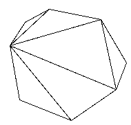
A chord is a line segment connecting any two vertices. A chord splits the polygon into two smaller polygons. Note that a chord always divides a convex polygon into two convex polygons.

A triangulation of a polygon can be thought of as a set of chords that divide the polygon into triangles such that no two chords intersect (except possibly at a vertex). This is a triangulation of the same polygon:

An optimal triangulation is one that minimizes some cost function of the triangles. A common cost function is the sum of the lengths of the legs of the triangles, i.e.

cost (<v_i, v_j, v_k>) = |v_i,v_j| + |v_j, v_k| + |v_i,v_k|

(where |a, b| is the Euclidean distance from point a to point b). We'll use this function for the discussion, although any function will work with the dynamic programming algorithm presented.

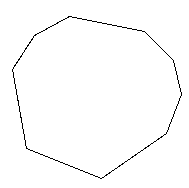
We would like to find, given a convex polygon and cost function over its vertices, the cost of an optimal triangulation of it. We would also like to get the structure of the triangulation itself as a list of triples of vertices.

This problem has a nice recursive substructure, a prerequisite for a dynamic programming algorithm. The idea is to divide the polygon into three parts: a single triangle, the sub-polygon to the left, and the sub-polygon to the right. We try all possible divisions like this until we find the one that minimizes the cost of the triangle plus the cost of the triangulation of the two sub-polygons. Where do we get the cost of triangulation of the two sub-polygons? Recursively, of course! The base case of the recursion is a line segment (i.e., a polygon with zero area), which has cost 0.

Let's define a function based on this intuitive notion. Let t(i, j) be the cost of an optimal triangulation of the polygon <v_i-1, v_i, v_i+1, ... , v_j>. So
t(i, j) =

0, if i=j
min_i<=k<=j-1 { t(i,k) + t(k+1,j) + cost (<v_i-1, v_k, v_j>)} if i < j

What's that say in English? If we just have a line segment, that is, we're just looking at the "polygon" <v_i-1, v_j>, so i=j, then t(i, j) is just 0. Otherwise, we let k go from i to j-1, looking at the sum of the costs of all triangles <v_i-1, v_k, v_j> and all polygons <v_i-1, ..., v_k> and <v_k+1, ..., v_j> and finding the minimum. Then t(1, n) is the cost of an optimal triangulation for the entire polygon.

More English, please? We just look at all possible triangles and leftover smaller polygons and pick the configuration that minimizes the cost.

We could write a recursive function in pseudocode right now, but it would be pretty inefficient. How inefficient? Well, remember the inefficient Fibonacci recursive function that took exponential time? It did only two recursive calls per invokation. This one does up to n recursive calls per invokation. This is a lot worse. There's no simple analysis, but since all possible triangulations will be explored by this method, a lower bound is same as the one given for an isomorphic problem in your book, about (4ⁿ / n^3/2). Yikes.

This situation is perfectly suited for dynamic programming. There are many redundant computations done. Each time we find a value for t(i, j), we can just stick that value into a two-dimensional array and never have to compute it again.

Here is the algorithm to compute the value of an optimal triangulation of a polygon given as an array V[0..n] of vertices. The array memo_t is an n by n array of real numbers initialized to -1. We must be careful to do arithmetic on vertex indices modulo n+1, to avoid going outside the array:

Triangulate (V)
	weight = t (1, n)
	print "the weight is" weight

t (i, j)
	if i == j then return 0
	if memo_t[i][j] != -1 then return memo_t[i][j]
	min = infinity
	for k in i..j-1 do
		x = t (i, k) + t (k+1 (mod n+1), j) 
			+ cost (<v[i-1 (mod n+1)], v[k], v[j]>)
		if x < min then min = x
	end for
	memo_t[i][j] = min
	return min

This takes (n²) storage because of the big array, and (n³) time since we have a function that does n things on n² array elements.

But this only tells us the value of an optimal solution? How do we find the structure, i.e., a list of triangles we can draw to actually triangulate the polygon? We can modify the memo_t array to be an array of pairs (c, k) where c is the minimum cost and k is the index of the vertex where the minimum cost was found. Then change the if statement above to:

		if x < min then 
			min = x
			mink = k
		end if

and the memo_t assignment to:

	memo_t[i][j].c = min
	memo_t[i][j].k = mink

Once we find the optimal cost, we have a history recorded in the array of a best vertex to do the recursive triangulations at each step. ("A" best, not "the" best, since there could have been two equally optimal vertices at any step.) We can print the list of triangles as triples of vertex indices using another recursive algorithm:

Print-Triangulation (i, j)
	if i != j then
		print i-1 (mod n+1), memo_t[i][j].k, j
		Print-Triangulation (i, memo_t[i][j].k)
		Print-Triangulation (memo_t[i][j].k+1 (mod n+1), j)
	end if

Then listing the triangles is just a call to Print-Triangulation (1, n). We can think of the triangulation procedure as mapping out a binary tree where the nodes are the minimal k's and the left and right children are the leftover polygons to triangulate. This algorithm is simply a preorder traversal of that tree, and works in

(n) time (since the number of triangles printed is exactly n-2).