Subsection 3.2.5 In practice, MGS is more accurate
¶In theory, all Gram-Schmidt algorithms discussed in the previous sections are equivalent in the sense that they compute the exact same QR factorizations when exact arithmetic is employed. In practice, in the presense of round-off error, the orthonormal columns of \(Q \) computed by MGS are often "more orthonormal" than those computed by CGS. We will analyze how round-off error affects linear algebra computations in the second part of the ALAFF. For now you will investigate it with a classic example.
When storing real (or complex) valued numbers in a computer, a limited accuracy can be maintained, leading to round-off error when a number is stored and/or when computation with numbers is performed. Informally, the machine epsilon (also called the unit roundoff error) is defined as the largest positive number, \(\epsilon_{\rm mach} \text{,}\) such that the stored value of \(1 + \epsilon_{\rm mach} \) is rounded back to \(1 \text{.}\)
Now, let us consider a computer where the only error that is ever incurred is when
is computed and rounded to \(1 \text{.}\)
Homework 3.2.5.1.
Let \(\epsilon = \sqrt{\epsilon_{\rm mach}} \) and consider the matrix
By hand, apply both the CGS and the MGS algorithms with this matrix, rounding \(1 + \epsilon_{\rm mach} \) to \(1\) whenever encountered in the calculation.
Upon completion, check whether the columns of \(Q\) that are computed are (approximately) orthonormal.
The complete calculation is given by
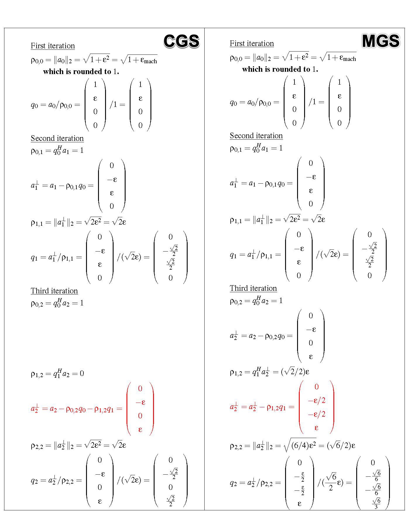
CGS yields the approximate matrix
while MGS yields
Clearly, they don't compute the same answer.
If we now ask the question "Are the columns of \(Q\) orthonormal?" we can check this by computing \(Q^H Q \text{,}\) which should equal \(I \text{,}\) the identity.
-
For CGS:
\begin{equation*} \begin{array}{l} Q^H Q \\ ~~~=~~~~ \\ \left( \begin{array}{c | c | c } 1 \amp 0 \amp 0 \\ \epsilon \amp -\frac{\sqrt{2}}{2} \amp -\frac{\sqrt{2}}{2} \\ 0 \amp \frac{\sqrt{2}}{2} \amp 0 \\ 0 \amp 0 \amp \frac{\sqrt{2}}{2} \end{array} \right)^H \left( \begin{array}{c | c | c } 1 \amp 0 \amp 0 \\ \epsilon \amp -\frac{\sqrt{2}}{2} \amp -\frac{\sqrt{2}}{2} \\ 0 \amp \frac{\sqrt{2}}{2} \amp 0 \\ 0 \amp 0 \amp \frac{\sqrt{2}}{2} \end{array} \right) \\ ~~~=~~~~\\ \left( \begin{array}{c c c } 1+\epsilon_{\rm mach} \amp - \frac{\sqrt{2}}{2} \epsilon \amp - \frac{\sqrt{2}}{2} \epsilon \\ - \frac{\sqrt{2}}{2} \epsilon \amp 1 \amp \frac{1}{2} \\ - \frac{\sqrt{2}}{2} \epsilon \amp \frac{1}{2} \amp 1 \\ \end{array} \right) . \end{array} \end{equation*}Clearly, the computed second and third columns of \(Q \) are not mutually orthonormal.
What is going on? The answer lies with how \(a_2^\perp \) is computed in the last step \(a_2^\perp := a_2 - ( q_0^H a_2 ) q_0 - ( q_1^H a_2 ) q_1\text{.}\) Now, \(q_0 \) has a relatively small error in it and hence \(q_0^H a_2 q_0 \) has a relatively small error in it. It is likely that a part of that error is in the direction of \(q_1 \text{.}\) Relative to \(q_0^H a_2 q_0 \text{,}\) that error in the direction of \(q_1 \) is small, but relative to \(a_2 - q_0^H a_2 q_0 \) it is not. The point is that then \(a_2 - q_0^H a_2 q_0 \) has a relatively large error in it in the direction of \(q_1 \text{.}\) Subtracting \(q_1^H a_2 q_1 \) does not fix this and since in the end \(a_2^\perp\) is small, it has a relatively large error in the direction of \(q_ 1 \text{.}\) This error is amplified when \(q_2 \) is computed by normalizing \(a_2^\perp \text{.}\)
-
For MGS:
\begin{equation*} \begin{array}{l} Q^H Q \\ ~~~=~~~~ \\ \left( \begin{array}{c | c | c } 1 \amp 0 \amp 0 \\ \epsilon \amp -\frac{\sqrt{2}}{2} \amp -\frac{\sqrt{6}}{6} \\ 0 \amp \frac{\sqrt{2}}{2} \amp -\frac{\sqrt{6}}{6} \\ 0 \amp 0 \amp \frac{\sqrt{6}}{3} \end{array} \right)^H \left( \begin{array}{c | c | c } 1 \amp 0 \amp 0 \\ \epsilon \amp -\frac{\sqrt{2}}{2} \amp -\frac{\sqrt{6}}{6} \\ 0 \amp \frac{\sqrt{2}}{2} \amp -\frac{\sqrt{6}}{6} \\ 0 \amp 0 \amp \frac{\sqrt{6}}{3} \end{array} \right) \\ ~~~=~~~~\\ \left( \begin{array}{c c c } 1+\epsilon_{\rm mach} \amp - \frac{\sqrt{2}}{2} \epsilon \amp - \frac{\sqrt{6}}{6} \epsilon \\ - \frac{\sqrt{2}}{2} \epsilon \amp 1 \amp 0 \\ - \frac{\sqrt{6}}{6} \epsilon \amp 0 \amp 1 \\ \end{array} \right) . \end{array} \end{equation*}Why is the orthogonality better? Consider the computation of \(a_2^\perp := a_2 - ( q_1^H a_2 ) q_1 \text{:}\)
\begin{equation*} a_2^\perp := a_2^\perp - q_1^H a_2^\perp q_1 = [ a_2 - ( q_0^H a_2 ) q_0 ] - ( q_1^H [ a_2 - ( q_0^H a_2 ) q_0 ] ) q_1. \end{equation*}This time, if \(a_2 - q_0^H a_2^\perp q_0 \) has an error in the direction of \(q_1 \text{,}\) this error is subtracted out when \(( q_1^H a_2^\perp) q_1 \) is subtracted from \(a_2^\perp \text{.}\) This explains the better orthogonality between the computed vectors \(q_1 \) and \(q_2 \text{.}\)
We have argued via an example that MGS is more accurate than CGS. A more thorough analysis is needed to explain why this is generally so.