Section 2.3 Vector registers and vector instructions
¶Unit 2.3.1 A simple model of memory and registers
For computation to happen, input data must be brought from memory into registers and, sooner or later, output data must be written back to memory.
For now let us make the following assumptions:
Our processor has only one core.
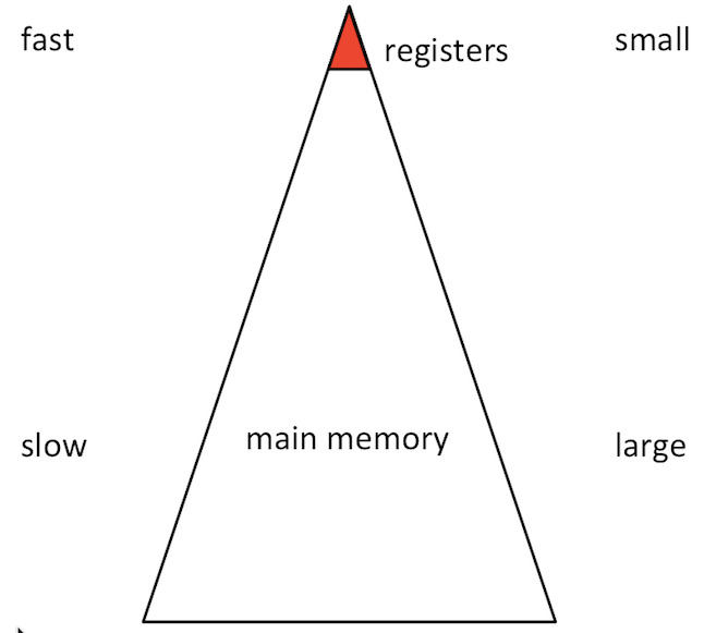
That core only has two levels of memory: registers and main memory.
Moving data between main memory and registers takes time \(\beta \) per double.
The registers can hold 64 doubles.
Performing a flop with data in registers takes time \(\gamma_R \text{.}\)
Data movement and computation cannot overlap.
Later, we will change some of these assumptions.
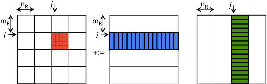
Given that the registers can hold 64 doubles, let's first consider blocking \(C \text{,}\) \(A \text{,}\) and \(B \) into \(4 \times 4 \) submatrices. In other words, consider the example from Unit 2.2.1 with \(m_R = n_R = k_R = 4 \text{.}\) This means \(3 \times 4 \times 4 = 48 \) registers are being used for storing the submatrices. (Yes, we are not using all registers. We'll get to that later.) Let us call the routine that computes with three blocks "the kernel". Thus, the blocked algorithm is a triple-nested loop around a call to this kernel:
\begin{equation*}
\begin{array}{l}
{\bf for~} i := 0, \ldots , M-1 \\
~~~ {\bf for~} j := 0, \ldots , N-1 \\
~~~ ~~~ {\bf for~} p := 0, \ldots , K-1 \\
~~~ ~~~ ~~~ {\rm Load~} C_{i,j} , A_{i,p} , {\rm ~and~} B_{p,j} \\
~~~ ~~~ ~~~ C_{i,j} := A_{i,p} B_{p,j} + C_{i,j} \\
~~~ ~~~ ~~~ {\rm Store~} C_{i,j} \\
~~~ ~~~ {\bf end} \\
~~~ {\bf end} \\
{\bf end}
\end{array}
\end{equation*}
as illustrated by
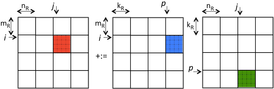
The time required to complete this algorithm can be estimated as
\begin{equation*}
\begin{array}{l}
M N K ( 2 m_R n_R k_R ) \gamma_R+ M N K ( 2 m_R n_R + m_R k_R + k_R n_R ) \beta\\
~~~~= 2 m n k \gamma_R+ m n k ( \frac{2}{k_R} +
\frac{1}{n_R} + \frac{1}{m_R} ) \beta,
\end{array}
\end{equation*}
since \(M = m/m_R\) , \(N = n/n_R \text{,}\) and \(K = k/k_R \text{,}\)
We next recognize that since the loop indexed with \(p\) is the inner-most loop, the loading and storing of \(C_{i,j} \) does not need to happen before every call to the kernel, yielding the algorithm
\begin{equation*}
\begin{array}{l}
{\bf for~} i := 0, \ldots , M-1 \\
~~~ {\bf for~} j := 0, \ldots , N-1 \\
~~~ ~~~ {\rm Load~} C_{i,j} \\
~~~ ~~~ {\bf for~} p := 0, \ldots , K-1 \\
~~~ ~~~ ~~~ {\rm Load~} A_{i,p} , {\rm ~and~} B_{p,j} \\
~~~ ~~~ ~~~ C_{i,j} := A_{i,p} B_{p,j} + C_{i,j} \\
~~~ ~~~ {\bf end} \\
~~~ ~~~ {\rm Store~} C_{i,j} \\
~~~ {\bf end} \\
{\bf end}
\end{array}
\end{equation*}
as illustrated by
Compute the estimated cost of the last algorithm.
Solution
\begin{equation*}
\begin{array}{l}
M N K ( 2 m_R n_R k_R ) \gamma_R
+ \left[ M N ( 2 m_R n_R )
+ M N K (m_R k_R + k_R n_R )\right] \beta\\
~~~= 2 m n k \gamma_R+ \left[ 2 m n + m n k (
\frac{1}{n_R} + \frac{1}{m_R} ) \right] \beta.
\end{array}
\end{equation*}
Homework 2.3.3
In directory Assignments/Week2/C copy the file Assignments/Week2/C/Gemm_IJP_mbxnbxkb.c into Gemm_IJ_mbxnbxk.c and remove the loop indexed by P. View its performance with Assignments/Week2/C/data/Plot_Blocked_MMM.mlx
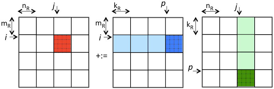
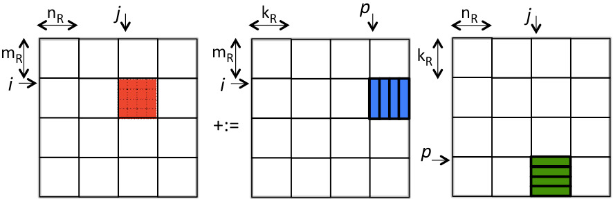
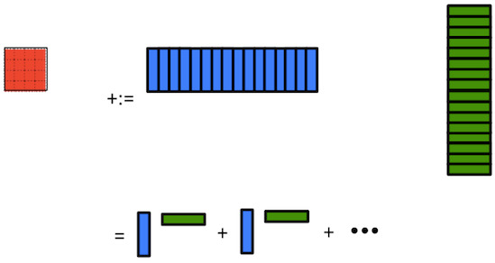
Now, if the submatrix \(C_{i,j} \) were larger (i.e., \(m_R \) and \(n_R \) were larger), then the overhead can be reduced. Obviously, we can use more registers (we are only storing 48 of a possible 64 doubles in registers when \(m_R = n_R = k_R = 4 \)). However, let's first discuss how to require fewer than 48 doubles to be stored while keeping \(m_R = n_R = k_R = 4 \text{.}\) Recall from Week 1 that if the P loop of matrix-matrix multiplication is the outer-most loop, then the inner two loops implement a rank-1 update. If we do this for the kernel, then the result is illustrated by
If we now consider the computation

void Gemm_IJP_P_bli_dger( int m, int n, int k, double *A, int ldA,
			  double *B, int ldB, double *C, int ldC )
{
  for ( int i=0; i\lt;m; i+=MR ) /* m assumed to be multiple of MR */
    for ( int j=0; j\lt;n; j+=NR ) /* n assumed to be multiple of NR */
      for ( int p=0; p\lt;k; p+=KR ) /* k assumed to be multiple of KR */
	Gemm_P_bli_dger( MR, NR, KR, &alpha( i,p ), ldA,
			 &beta( p,j ), ldB, &gamma( i,j ), ldC );
}

void Gemm_P_bli_dger( int m, int n, int k, double *A, int ldA,
		      double *B, int ldB, double *C, int ldC )
{
  double d_one = 1.0;

  for ( int p=0; p\lt;k; p++ )
    bli_dger( BLIS_NO_CONJUGATE, BLIS_NO_CONJUGATE, m, n, &d_one,
              &alpha( 0,p ), 1, &beta( p,0 ), ldB, C, 1, ldC, NULL );
}
\begin{center}
	\begin{minipage}{\textwidth}
		\lstinputlisting[numbers=left,firstnumber=26,language=C, firstline=26,
		title=\lstname]{Assignments/Week2/C/Gemm_IJ_P_bli_dger.c}
	\end{minipage}
	\end{center}
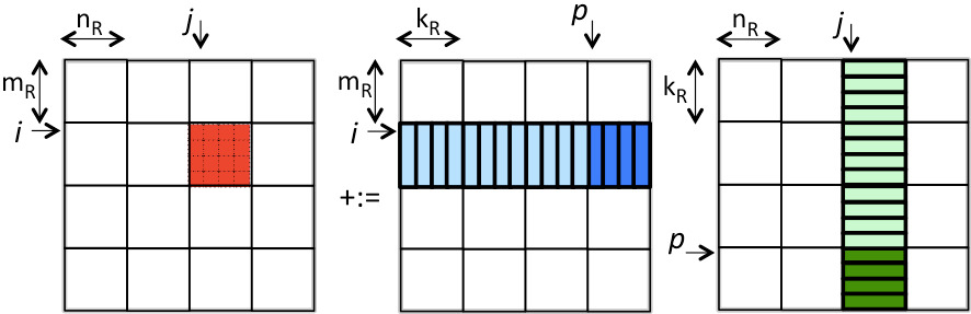
What we now recognize is that matrices \(A \) and \(B\) need not be partitioned into \(m_R \times k_R \) and \(k_R \times n_R \) submatrices (respectively). Instead, \(A\) can be partitioned into \(m_R \times k\) row panels and \(B\) into \(k \times n_R \) column panels:
Bringing \(A_{i,p} \) one column at a time into registers and \(B_{p,j} \) one row at a time into registers does not change the cost of reading that data. So, the cost of the resulting approach is still estimated as
\begin{equation*}
\begin{array}{l}
M N K ( 2 m_R n_R k_R ) \gamma_R
+ \left[ M N ( 2 m_R n_R )
+ M N K (m_R k_R + k_R n_R )\right] \beta \\
~~~= 2 m n k \gamma_R+ \left[ 2 m n + m n k (
\frac{1}{n_R} + \frac{1}{m_R} ) \right] \beta.
\end{array}
\end{equation*}
We can arrive at the same algorithm by partitioning
\begin{equation*}
C = \left( \begin{array}{c | c | c | c }
C_{0,0} \amp C_{0,1} \amp \cdots \amp C_{0,N-1} \\ \hline
C_{1,0} \amp C_{1,1} \amp \cdots \amp C_{1,N-1} \\ \hline
\vdots \amp \vdots \amp \amp \vdots \\ \hline
C_{M-1,0} \amp C_{M,1} \amp \cdots \amp C_{M-1,N-1}
\end{array} \right),
A = \left( \begin{array}{c }
A_{0} \\ \hline
A_{1} \\ \hline
\vdots \\ \hline
A_{M-1}
\end{array} \right),
\end{equation*}
and
\begin{equation*}
B = \left( \begin{array}{c | c | c | c }
B_{0} \amp B_{1} \amp \cdots \amp B_{0,N-1}
\end{array} \right),
\end{equation*}
where \(C_{i,j} \) is \(m_R \times n_R \text{,}\) \(A_i \) is \(m_R \times k \text{,}\) and \(B_j \) is \(k \times n_R \text{.}\) Then computing \(C := A B + C \) means updating \(C_{i,j} := A_i B_j + C_{i,j} \) for all \(i, j \text{:}\)
\begin{equation*}
\begin{array}{l}
\begin{array}{l}
{\bf for~} i := 0, \ldots , M-1 \\[0.05in]
~~~
\left. \begin{array}{l}
{\bf for~} j := 0, \ldots , N-1 \\[0.05in]
~~~ ~~~
\left. \begin{array}{l}
C_{i,j} := A_i B_j + C_{i,j}
\end{array} \right. ~~~ \mbox{Computed with the microkernel} \\[0.1in]
~~~ {\bf end}
\end{array}\right. \\[0.1in]
{\bf end}
\end{array}
\end{array}
\end{equation*}
Obviously, the order of the two loops can be switched. Again, the computation \(C_{i,j} := A_i B_j + C_{i,j} \) where \(C_{i,j} \) fits in registers now becomes what we will call the microkernel.
Homework 2.3.6
In directory Assignments/Week2/C examine the file Assignments/Week2/C/Gemm_IJ_P_bli_dger.c Execute it with make IJ_P_bli_dger and view its performance with Assignments/Week2/C/data/Plot_Blocked_MMM.mlx
Unit 2.3.2 Instruction-level parallelism
¶As the reader should have noticed by now, in matrix-matrix multiplication for every floating point multiplication a corresponding floating point addition is encountered to accumulate the result. For this reason, such floating point computations are usually cast in terms of fused multiply add ( FMA) operations, performed by a floating point unit (FPU) of the core.
What is faster than computing one FMA at a time? Computing multiple FMAs at a time! To accelerate computation, modern cores are equipped with vector registers, vector instructions, and vector FPUs that can simultaneously perform multiple FMA operations. This is called instruction-level parallelism.
In this section, we are going to use Intel's vector intrinsic instructions for Intel's AVX instruction set to illustrate the ideas. Vector intrinsics are supported in the C programming language for performing these vector instructions. We illustrate how the intrinsic operations are used by incorporating them into an implemention of the microkernel for the case where \(m_R \times n_R = 4 \times 4 \text{.}\) Thus, for the remainder of this unit, \(C \) is \(m_R \times n_R = 4 \times 4 \text{,}\) \(A \) is \(m_R \times k = 4 \times k \text{,}\) and \(B \) is \(k \times n_R = k \times 4 \text{.}\)
Now, \(C +:= A B \) when \(C \) is \(4 \times 4 \) translates to the computation
\begin{equation*}
\begin{array}{l}
\left( \begin{array}{c | c | c | c}
\gamma_{0,0} \amp \gamma_{0,1} \amp \gamma_{0,2} \amp \gamma_{0,3} \\
\gamma_{1,0} \amp \gamma_{1,1} \amp \gamma_{1,2} \amp \gamma_{1,3} \\
\gamma_{2,0} \amp \gamma_{2,1} \amp \gamma_{2,2} \amp \gamma_{2,3} \\
\gamma_{3,0} \amp \gamma_{3,1} \amp \gamma_{3,2} \amp \gamma_{3,3}
\end{array}\right)
\\
~~~ +:= \left( \begin{array}{c | c | c }
\alpha_{0,0} \amp \color{red} \alpha_{0,1} \amp \cdots \\
\alpha_{1,0} \amp \color{red} \alpha_{1,1} \amp \cdots \\
\alpha_{2,0} \amp \color{red} \alpha_{2,1} \amp \cdots \\
\alpha_{3,0} \amp \color{red} \alpha_{3,1} \amp \cdots
\end{array}\right)
\left( \begin{array}{c c c c}
\beta_{0,0} \amp \beta_{0,1} \amp \beta_{0,2} \amp \beta_{0,3} \\
\beta_{1,0} \amp \color{blue} \beta_{1,1} \amp \beta_{1,2} \amp \beta_{1,3} \\
\vdots \amp \vdots \amp \vdots \amp \vdots
\end{array}\right) \\
~~~ =
\left(\begin{array}{c | c | c | c }
\alpha_{0,0} \beta_{0,0} + {\color{red} \alpha_{0,1}} \beta_{1,0} + \cdots
\amp
\alpha_{0,0} \beta_{0,1} + {\color{red} \alpha_{0,1}} {\color{blue} \beta_{1,1}} + \cdots
\amp
\alpha_{0,0} \beta_{0,2} + {\color{red} \alpha_{0,1}} \beta_{1,2} + \cdots
\amp
\alpha_{0,0} \beta_{0,2} + {\color{red} \alpha_{0,1}} \beta_{1,2} + \cdots
\\
\alpha_{1,0} \beta_{0,0} + {\color{red} \alpha_{1,1}} \beta_{1,0} + \cdots
\amp
\alpha_{1,0} \beta_{0,1} + {\color{red} \alpha_{1,1}} {\color{blue} \beta_{1,1}} + \cdots
\amp
\alpha_{1,0} \beta_{0,2} + {\color{red} \alpha_{1,1}} \beta_{1,2} + \cdots
\amp
\alpha_{1,0} \beta_{0,3} + {\color{red} \alpha_{1,1}} \beta_{1,3} + \cdots
\\
\alpha_{2,0} \beta_{0,0} + {\color{red} \alpha_{2,1}} \beta_{1,0} + \cdots
\amp
\alpha_{2,0} \beta_{0,1} + {\color{red} \alpha_{2,1}} {\color{blue} \beta_{1,1}} + \cdots
\amp
\alpha_{2,0} \beta_{0,2} + {\color{red} \alpha_{2,1}} \beta_{1,2} + \cdots
\amp
\alpha_{2,0} \beta_{0,3} + {\color{red} \alpha_{2,1}} \beta_{1,3} + \cdots
\\
\alpha_{3,0} \beta_{0,0} + {\color{red} \alpha_{3,1}} \beta_{1,0} + \cdots
\amp
\alpha_{3,0} \beta_{0,1} + {\color{red} \alpha_{3,1}} {\color{blue} \beta_{1,1}} + \cdots
\amp
\alpha_{3,0} \beta_{0,2} + {\color{red} \alpha_{3,1}} \beta_{1,2} + \cdots
\amp
\alpha_{3,0} \beta_{0,3} + {\color{red} \alpha_{3,1}} \beta_{1,3} + \cdots
\end{array}
\right)
\\
~~~ =
\left( \begin{array}{c}
\alpha_{0,0} \\
\alpha_{1,0} \\
\alpha_{2,0} \\
\alpha_{3,0}
\end{array}\right)
\left( \begin{array}{c c c c}
\beta_{0,0} \amp \beta_{0,1} \amp \beta_{0,2} \amp \beta_{0,3} \\
\end{array}\right)
+
\left( \begin{array}{c c c c}
{\color{red} \alpha_{0,1}} \\
{\color{red} \alpha_{1,1}} \\
{\color{red} \alpha_{2,1}} \\
{\color{red} \alpha_{3,1}}
\end{array}\right)
\left( \begin{array}{c c c c}
\beta_{1,0} \amp {\color{blue} \beta_{1,1}} \amp \beta_{1,2} \amp \beta_{1,3} \\
\end{array}\right)
+ \cdots
\end{array}
\end{equation*}
Thus, updating \(4 \times 4 \) matrix \(C \) can be implemented as a loop around rank-1 updates:
\begin{equation*}
\begin{array}{l}
{\bf for~} p = 0, \ldots, k-1\\
~~~
\left( \begin{array}{c | c | c | c}
\gamma_{0,0} \amp \gamma_{0,1} \amp \gamma_{0,2} \amp \gamma_{0,3} \\
\gamma_{1,0} \amp \gamma_{1,1} \amp \gamma_{1,2} \amp \gamma_{1,3} \\
\gamma_{2,0} \amp \gamma_{2,1} \amp \gamma_{2,2} \amp \gamma_{2,3} \\
\gamma_{3,0} \amp \gamma_{3,1} \amp \gamma_{3,2} \amp \gamma_{3,3}
\end{array}\right)
+:=
\left( \begin{array}{c c c c}
\alpha_{0,p} \\
\alpha_{1,p} \\
\alpha_{2,p} \\
\alpha_{3,p}
\end{array}\right)
\left( \begin{array}{c c c c}
\beta_{p,0} \amp \beta_{p,1} \amp \beta_{p,2} \amp \beta_{p,3} \\
\end{array}\right)
\\
{\bf endfor}
\end{array}
\end{equation*}
or, equivalently to emphasize computations with vectors,
\begin{equation*}
\begin{array}{l}
{\bf for~} p = 0, \ldots, k-1 \\
~~~
\left( \begin{array}{c | c | c | c}
\begin{array}{c c c c}
\gamma_{0,0} +:= \alpha_{0,p} \times \beta_{p,0} \\
\gamma_{1,0} +:= \alpha_{1,p} \times \beta_{p,0} \\
\gamma_{2,0} +:= \alpha_{2,p} \times \beta_{p,0} \\
\gamma_{3,0} +:= \alpha_{3,p} \times \beta_{p,0}
\end{array}
\amp
\begin{array}{c c c c}
\gamma_{0,1} +:= \alpha_{0,p} \times \beta_{p,1} \\
\gamma_{1,1} +:= \alpha_{1,p} \times \beta_{p,1} \\
\gamma_{2,1} +:= \alpha_{2,p} \times \beta_{p,1} \\
\gamma_{3,1} +:= \alpha_{3,p} \times \beta_{p,1}
\end{array}
\amp
\begin{array}{c c c c}
\gamma_{0,2} +:= \alpha_{0,p} \times \beta_{p,2} \\
\gamma_{1,2} +:= \alpha_{1,p} \times \beta_{p,2} \\
\gamma_{2,2} +:= \alpha_{2,p} \times \beta_{p,2} \\
\gamma_{3,2} +:= \alpha_{3,p} \times \beta_{p,2}
\end{array}
\amp
\begin{array}{c c c c}
\gamma_{0,3} +:= \alpha_{0,p} \times \beta_{p,3} \\
\gamma_{1,3} +:= \alpha_{1,p} \times \beta_{p,3} \\
\gamma_{2,3} +:= \alpha_{2,p} \times \beta_{p,3} \\
\gamma_{3,3} +:= \alpha_{3,p} \times \beta_{p,3}
\end{array}
\end{array}\right)
\\
{\bf endfor}
\end{array}
\end{equation*}
This, once again, shows how matrix-matrix multiplication can be cast in terms of a sequence of rank-1 updates, and that a rank-1 update can be implemented in terms of axpy operations with columns of \(C \text{.}\)
#include <stdio.h>
#include <stdlib.h>

#define alpha( i,j ) A[ (j)*ldA + (i) ]   // map alpha( i,j ) to array A
#define beta( i,j )  B[ (j)*ldB + (i) ]   // map beta( i,j ) to array B
#define gamma( i,j ) C[ (j)*ldC + (i) ]   // map gamma( i,j ) to array C

#define MR 4
#define NR 4

void Gemm_IJ_4x4Kernel( int, int, int, double *, int, double *, int, double *, int );

void Gemm_4x4Kernel( int, double *, int, double *, int, double *, int );

void MyGemm( int m, int n, int k, double *A, int ldA,
		  double *B, int ldB, double *C, int ldC )
{
  if ( m % MR != 0 || n % NR != 0 ){
    printf( "m and n must be multiples of MR and NR, respectively \n" );
    exit( 0 );
  }

  for ( int i=0; i<m; i+=MR ) /* m is assumed to be a multiple of MR */
    for ( int j=0; j<n; j+=NR ) /* n is assumed to be a multiple of NR */
      Gemm_4x4Kernel( k, &alpha( i,0 ), ldA, &beta( 0,j ), ldB, &gamma( i,j ), ldC );
}

#include<immintrin.h>

void Gemm_4x4Kernel( int k, double *A, int ldA, double *B, int ldB,
		double *C, int ldC )
{
  /* Declare vector registers to hold 4x4 C and load them */
  __m256d gamma_0123_0 = _mm256_loadu_pd( &gamma( 0,0 ) );
  __m256d gamma_0123_1 = _mm256_loadu_pd( &gamma( 0,1 ) );
  __m256d gamma_0123_2 = _mm256_loadu_pd( &gamma( 0,2 ) );
  __m256d gamma_0123_3 = _mm256_loadu_pd( &gamma( 0,3 ) );

  for ( int p=0; p<k; p++ ){
    /* Declare vector register for load/broadcasting beta( b,j ) */
    __m256d beta_p_j;

    /* Declare a vector register to hold the current column of A and load
       it with the four elements of that column. */
    __m256d alpha_0123_p = _mm256_loadu_pd( &alpha( 0,p ) );

    /* Load/broadcast beta( p,0 ). */
    beta_p_j = _mm256_broadcast_sd( &beta( p, 0) );

    /* update the first column of C with the current column of A times
       beta ( p,0 ) */
    gamma_0123_0 = _mm256_fmadd_pd( alpha_0123_p, beta_p_j, gamma_0123_0 );

    /* REPEAT for second, third, and fourth columns of C.  Notice that the
       current column of A needs not be reloaded. */


  }

  /* Store the updated results */
  _mm256_storeu_pd( &gamma(0,0), gamma_0123_0 );
  _mm256_storeu_pd( &gamma(0,1), gamma_0123_1 );
  _mm256_storeu_pd( &gamma(0,2), gamma_0123_2 );
  _mm256_storeu_pd( &gamma(0,3), gamma_0123_3 );
}
Assignments/Week2/C/Gemm_IJ_4x4Kernel.c).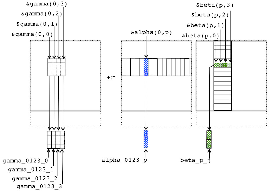
Now we translate this into code that employs vector instructions, given in Figure~Figure 2.3.7 and illustrated in Figure 2.3.8. To use the intrinsics, we start by including the header file immintrin.h.
#include<immintrin.h>
The declaration
__m256d gamma_0123_0 = _mm256_loadu_pd( &gamma( 0,0 ) );creates gamma_0123_0 as a variable that references a vector register with four double precision numbers and loads it with the four numbers that are stored starting at address &gamma( 0,0 ). In other words, it loads the vector register with the original values
\begin{equation*}
\left(
\begin{array}{c c c c}
\gamma_{0,0} \\
\gamma_{1,0} \\
\gamma_{2,0} \\
\gamma_{3,0}
\end{array}
\right).
\end{equation*}
This is repeated for the other three columns of \(C \text{:}\)
__m256d gamma_0123_1 = _mm256_loadu_pd( &gamma( 0,1 ) );
__m256d gamma_0123_2 = _mm256_loadu_pd( &gamma( 0,2 ) );
__m256d gamma_0123_3 = _mm256_loadu_pd( &gamma( 0,3 ) );
The loop in Figure 2.3.7 implements
\begin{equation*}
\begin{array}{l}
{\bf for~} p = 0, \ldots, k-1 \\
~~~
\left( \begin{array}{c | c | c | c}
\begin{array}{c c c c}
\gamma_{0,0} +:= \alpha_{0,p} \times \beta_{p,0} \\
\gamma_{1,0} +:= \alpha_{1,p} \times \beta_{p,0} \\
\gamma_{2,0} +:= \alpha_{2,p} \times \beta_{p,0} \\
\gamma_{3,0} +:= \alpha_{3,p} \times \beta_{p,0}
\end{array}
\amp
\begin{array}{c c c c}
\gamma_{0,1} +:= \alpha_{0,p} \times \beta_{p,1} \\
\gamma_{1,1} +:= \alpha_{1,p} \times \beta_{p,1} \\
\gamma_{2,1} +:= \alpha_{2,p} \times \beta_{p,1} \\
\gamma_{3,1} +:= \alpha_{3,p} \times \beta_{p,1}
\end{array}
\amp
\begin{array}{c c c c}
\gamma_{0,2} +:= \alpha_{0,p} \times \beta_{p,2} \\
\gamma_{1,2} +:= \alpha_{1,p} \times \beta_{p,2} \\
\gamma_{2,2} +:= \alpha_{2,p} \times \beta_{p,2} \\
\gamma_{3,2} +:= \alpha_{3,p} \times \beta_{p,2}
\end{array}
\amp
\begin{array}{c c c c}
\gamma_{0,3} +:= \alpha_{0,p} \times \beta_{p,3} \\
\gamma_{1,3} +:= \alpha_{1,p} \times \beta_{p,3} \\
\gamma_{2,3} +:= \alpha_{2,p} \times \beta_{p,3} \\
\gamma_{3,3} +:= \alpha_{3,p} \times \beta_{p,3}
\end{array}
\end{array}\right)
\\
{\bf endfor}
\end{array}
\end{equation*}
leaving the result in the vector registers. Each iteration starts by declaring vector register variable alpha_0123_p and loading it with the contents of
\begin{equation*}
\left(
\begin{array}{c c c c}
\alpha_{0,p} \\
\alpha_{1,p} \\
\alpha_{2,p} \\
\alpha_{3,p}
\end{array}
\right).
\end{equation*}
__m256d alpha_0123_p = _mm256_loadu_pd( &alpha( 0,p ) );Next, \(\beta_{p,0} \) is loaded into a vector register, broadcasting (duplicating) that value to each entry in that register:
beta_p_j = _mm256_broadcast_sd( &beta( p, 0) );(This variable is declared earlier in the routine.) The command
gamma_0123_0 = _mm256_fmadd_pd( alpha_0123_p, beta_p_j, gamma_0123_0 );then performs the computation
\begin{equation*}
\left(
\begin{array}{c c c c}
\gamma_{0,0} +:= \alpha_{0,p} \times \beta_{p,0} \\
\gamma_{1,0} +:= \alpha_{1,p} \times \beta_{p,0} \\
\gamma_{2,0} +:= \alpha_{2,p} \times \beta_{p,0} \\
\gamma_{3,0} +:= \alpha_{3,p} \times \beta_{p,0}
\end{array}
\right).
\end{equation*}
We leave it to the reader to add the commands that compute
\begin{equation*}
\left(
\begin{array}{c c c c}
\gamma_{0,1} +:= \alpha_{0,p} \times \beta_{p,1} \\
\gamma_{1,1} +:= \alpha_{1,p} \times \beta_{p,1} \\
\gamma_{2,1} +:= \alpha_{2,p} \times \beta_{p,1} \\
\gamma_{3,1} +:= \alpha_{3,p} \times \beta_{p,1}
\end{array}
\right),
\quad
\left(
\begin{array}{c c c c}
\gamma_{0,2} +:= \alpha_{0,p} \times \beta_{p,2} \\
\gamma_{1,2} +:= \alpha_{1,p} \times \beta_{p,2} \\
\gamma_{2,2} +:= \alpha_{2,p} \times \beta_{p,2} \\
\gamma_{3,2} +:= \alpha_{3,p} \times \beta_{p,2}
\end{array}
\right), \quad \mbox{and} \quad
\left(
\begin{array}{c c c c}
\gamma_{0,3} +:= \alpha_{0,p} \times \beta_{p,3} \\
\gamma_{1,3} +:= \alpha_{1,p} \times \beta_{p,3} \\
\gamma_{2,3} +:= \alpha_{2,p} \times \beta_{p,3} \\
\gamma_{3,3} +:= \alpha_{3,p} \times \beta_{p,3}
\end{array}
\right).
\end{equation*}
in Assignments/Week2/C/Gemm_IJ_4x4Kernel.c. Upon completion of the loop, the results are stored back into the original arrays with the commands
_mm256_storeu_pd( &gamma(0,0), gamma_0123_0 );
_mm256_storeu_pd( &gamma(0,1), gamma_0123_1 );
_mm256_storeu_pd( &gamma(0,2), gamma_0123_2 );
_mm256_storeu_pd( &gamma(0,3), gamma_0123_3 );
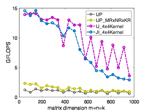
Homework 2.3.9
Complete the code in Assignments/Week2/C/Gemm_IJ_4x4Kernel.c View its performance with Assignments/Week2/C/data/Plot_MRxNR_Kernels.mlx
Homework 2.3.10
After completing it, copy Assignments/Week2/C/Gemm_IJ_4x4Kernel.c and reverse the I and J loops. View its performance with Assignments/Week2/C/data/Plot_Blocked matrix-matrix multiplication mlx
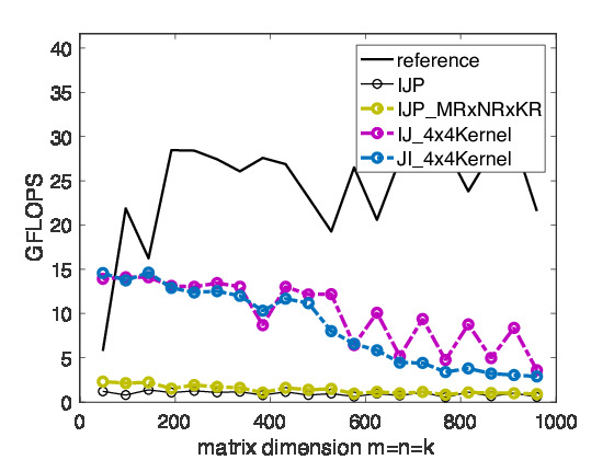
Remark 2.3.11
On Robert's laptop, we are starting to see some progress towards high performance, as illustrated in