Section 3.4 Further Tricks of the Trade
¶We now give a laundry list of further optimizations that can be tried.
Unit 3.4.1 Microkernels with different choices for microtile
¶As mentioned, there are many choices for \(m_R \times n_R \text{.}\) On the Haswell architecture, we focused on \(12 \times 4 \text{.}\) You may have discovered that \(8 \times 6\) works better.
Redo the last few exercises to create Gemm_Five_Loops_8x6Kernel.c Gemm_Five_Loops_Pack_8x6Kernel.c. Modify the Makefile and Live Script Plot_Five_Loops.mlx as appropriate.
Unit 3.4.2 Broadcasting elements of \(A\) and loading elements of \(B\)
¶So far, we have focused on choices for \(m_R \times n_R \) where \(m_R\) is a multiple of four. Before packing was added, this was because one loads into registers from contiguous memory and for this reason loading from \(A \text{,}\) four elements at a time, while broadcasting elements from \(B \) was natural becanuse of how data was mapped to memory using column-major order. After packing was introduced, one could also contemplate loading from \(B \) and broadcasting elements of \(A \text{,}\) which then also makes kernels like \(6 \times 8 \) possible. The problem is that this would mean performing a vector instruction with elements that are in rows of \(C \text{,}\) and hence when loading elements of \(C \) one would need to perform a transpose operation, and also when storing the elements back to memory.
There are reasons whey a \(6 \times 8 \) kernel edges out even a \(8 \times 6 \) kernel. On the surface, it may seem like this would require a careful reengineering of the five loops as well as the microkernel. However, there are tricks that can be played to make it much simpler than it seems.
Intuitively, if you store matrices by columns, leave the data as it is so stored, but then work with the data as if it is stored by rows, this is like computing with the transposes of the matrices. Now, mathematically, if
\begin{equation*}
C := A B + C
\end{equation*}
then
\begin{equation*}
C^T :=
( A B + C )^T =
( A B )^T + C^T = B^T A^T + C^T.
\end{equation*}
If you think about it: transposing a matrix is equivalent to viewing the matrix, when stored in column-major order, as being stored in row-major order.
Homework 3.4.2
Transform your favorite implementation of the five loops with packing into Gemm_Five_Loops_Pack_6x8Kernel.c. Modify the Makefile and Live Script Plot_Five_Loops.mlx as appropriate. }
Consider the simplest implementation for computing \(C := A B + C \) from Week 1:
#define alpha( i,j ) A[ (j)*ldA + i ]
#define beta( i,j )  B[ (j)*ldB + i ]
#define gamma( i,j ) C[ (j)*ldC + i ]

void MyGemm( int m, int n, int k, double *A, int ldA,
                    double *B, int ldB, double *C, int ldC )
{
  for ( int i=0; i<m; i++ )
    for ( int j=0; j<n; j++ )
      for ( int p=0; p<k; p++ )
        gamma( i,j ) += alpha( i,p ) * beta( p,j );
}
From this, a code that instead computes \(C^T := B^T A^T
+ C^T \text{,}\) with matrices still stored in column-major order, is given by #define alpha( i,j ) A[ (j)*ldA + i ]
#define beta( i,j ) B[ (j)*ldB + i ]
#define gamma( i,j ) C[ (j)*ldC + i ]
void MyGemm( int m, int n, int k, double *A, int ldA,
double *B, int ldB, double *C, int ldC )
{
for ( int i=0; i<m; i++ )
for ( int j=0; j<n; j++ )
for ( int p=0; p<k; p++ )
gamma( j,i ) += alpha( p,i ) * beta( j,p );
}
Notice how the roles of m and n are swapped and how working with the transpose replaces i,j with j,i, etc. However, we could have been clever: Instead of replacing i,j with j,i, etc., we could have instead swapped the order of these in the macro definitions: #define alpha( i,j ) becomes #define alpha( j,i ): #define alpha( j,i ) A[ (j)*ldA + i ]
#define beta( j,i ) B[ (j)*ldB + i ]
#define gamma( j,i ) C[ (j)*ldC + i ]
void MyGemm( int m, int n, int k, double *A, int ldA,
double *B, int ldB, double *C, int ldC )
{
for ( int i=0; i<m; i++ )
for ( int j=0; j<n; j++ )
for ( int p=0; p<k; p++ )
gamma( i,j ) += alpha( i,p ) * beta( p,j );
}
Next, we can get right back to our original triple-nested loop by swapping the roles of A and B: #define alpha( j,i ) A[ (j)*ldA + i ]
#define beta( j,i ) B[ (j)*ldB + i ]
#define gamma( j,i ) C[ (j)*ldC + i ]
void MyGemm( int m, int n, int k, double *B, int ldB,
double *A, int ldA, double *C, int ldC )
{
for ( int i=0; i<m; i++ )
for ( int j=0; j<n; j++ )
for ( int p=0; p<k; p++ )
gamma( i,j ) += alpha( i,p ) * beta( p,j );
}
The point is: Computing \(C := A B + C \) with these matrices stored by columns is the same as computing \(C
:= B A + C \) viewing the data as if stored by rows, making appropriate adjustments for the sizes of the matrix. With this insight, any matrix-matrix multiplication implementation we have encountered can be transformed into one that views the data as if stored by rows by redefining the macros that translate indexing into the arrays into how the matrices are stored, a swapping of the roles of \(A \) and \(B \text{,}\) and an adjustment to the sizes of the matrix.
Because we implement the packing with the macros, they actually can be used as is. What is left is to modify the inner kernel to use \(m_R \times n_R = 6 \times 8 \text{.}\)
Unit 3.4.3 Avoiding repeated memory allocations
¶In the final implementation that incorporates packing, at various levels workspace is allocated and deallocated multiple times. This can be avoided by allocating workspace immediately upon entering LoopFive (or in MyGemm). Alternatively, the space could be "statically allocated" as a global array of appropriate size. In "the real world" this is a bit dangerous: If an application calls multiple instances of matrix-matrix multiplication in parallel (e.g., using OpenMP about which we will learn next week), then these different instances may end up overwriting each other's data as they pack, leading to something called a "race condition." But for the sake of this course, it is a reasonable first step.
Unit 3.4.4 Alignment
¶There are alternative vector intrinsic routines that load vector registers under the assumption that the data being loaded is "32 byte aligned." This means that the address that specifies the four doubles being loaded is a multiple of 32.
Conveniently, loads of elements of \(A \) and \(B\) are from buffers into which the data was packed. By creating that buffer to be 32 byte aligned, we can ensure that all these loads are 32 byte aligned. Intel's intrinsic library has a special memory allocation routine specifically for this purpose.
Unit 3.4.5 Loop unrolling
¶There is some overhead that comes from having a loop in the microkernel. That overhead is in part due to the cost of updating the loop index p and the pointers to the buffers BlockA and PanelB. It is also possible that "unrolling" the loop will allow the compiler to rearrange more instructions in the loop and/or the hardware to better perform out-of-order computation because each iteration of the loop involves a branch instruction, where the branch depends on whether the loop is done. Branches get in the way of compiler optimizations and out-of-order computation by the CPU.
What is loop unrolling? In the case of the microkernel, unrolling the loop indexed by p by a factor two means that each iteration of that loop updates the microtile of \(C \) twice instead of once. In other words, each iteration of the unrolled loop performs two iterations of the original loop, and updates p+=2 instead of p++. Unrolling by a larger factor is the natural extension of this idea. Obviously, a loop that is unrolled requires some care in case the number of iterations was not a nice multiple of the unrolling factor. You may have noticed that our performance experiments always use problem sizes that are multiples of 48. This means that if you use a reasonable unrolling factor that divides into 48, you are probably going to be OK.
Similarly, one can unroll the loops in the packing routines.
Unit 3.4.6 Prefetching
¶Elements of \(\widetilde A \) in theory remain in the L2 cache. If you implemented the \(6 \times 8 \) kernel, you are using 15 out of 16 vector registers and the hardware almost surely prefetches the next element of \(\widetilde A \) into the L1 cache while computing with the current one. One can go one step further by using the last unused vector register as well, so that you use two vector registers to load/broadcast two elements of \(\widetilde A \text{.}\) The CPU of most modern codes will execute "out of order" which means that at the hardware level instructions are rescheduled so that a "stall" (a hickup in the execution because, for example, data is not available) is covered by other instructions. It is highly likely that this will result in the current computation overlapping with the next element from \(\widetilde A\) being prefetched (load/broadcast) into a vector register.
A second reason to prefetch is to overcome the latency to main memory for bringing in the next microtile of \(C \text{.}\) The Intel instruction set (and vector intrinsic library) includes instructions to prefetch data into an indicated level of cache. This is accomplished by calling the instruction
void _mm_prefetch(char *p, int i)
The argument *p gives the address of the byte (and corresponding cache line) to be prefetched.
-
The value i is the hint that indicates which level to prefetch to.
_MM_HINT_T0: prefetch data into all levels of the cache hierarchy.
_MM_HINT_T1: prefetch data into level 2 cache and higher.
_MM_HINT_T2: prefetch data into level 3 cache and higher, or an implementation-specific choice.
These are actually hints that a compiler can choose to ignore. In theory, with this a next microtile of \(C \) can be moved into a more favorable memory layer while a previous microtile is being updated. In theory, the same mechanism can be used to bring a next micro-panel of \(\widetilde B \text{,}\) which itself is meant to reside in the L3 cache, into the L1 cache during computation with a previous such micro-panel. In practice, we did not manage to make this work. It may work better to use equivalent instructions with in-lined assembly code.
For additional information, you may want to consult the Intel (R) 64 and IA-32 Architectures Software Developer’s Manual. This is a very long document... You will not want to print it.
Unit 3.4.7 Different cache block parameters
¶Choosing all blocking parameters carefully is likely to improve performance. Some believe that one should just try all parameters to determine them empirically. Some of our collaborators have shown that a careful analysis can yield near optimal choices:
Tze Meng Low, Francisco D. Igual, Tyler M. Smith, and Enrique S. Quintana-Orti. Analytical Modeling is Enough for High Performance BLIS. ACM Transactions on Mathematical Software, Volume 43 Issue 2, September 2016.
If you don't have access to ACM's publications, you can read an early draft.
Unit 3.4.8 Using in-lined assembly code
¶Even more control over where what happens from using in-lined assembly code. This will allow prefetching and how registers are used to be made more explicit. (The compiler often changes the order of the operations even when intrinsics are used in C.) Details go beyond this course. You may want to look at the href="https://github.com/flame/blis/blob/master/kernels/haswell/3/old/bli_gemm_haswell_asm_d6x8.c"> BLIS microkernel for the Haswell achitecture, implemented with in-lined assembly code.