Multi-scale Bio-Modeling and
Visualization
Project Notes: Modeling the
Neuro-Muscular Junction
Last Update
Overview
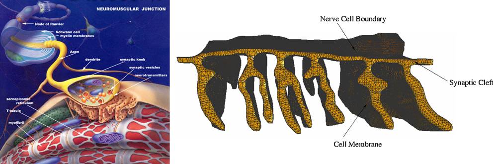
In this project we want to model the
neuro-muscular junction (see Figure 1). By modeling we mean properly placing
the entities involved in the physiological activity. In essence, it is a
geometric modeling exercise and for the time being we will focus on static
modeling, i.e., we will consider a snapshot and place the molecules -
Acetylcholine receptor (AchR) on the thickened cell membrane and
Acetylcholinesterase (AchE) in the synaptic cleft which is the volume entrapped
between the nerve cells and the cell membranes (see Figure 2 for an
example result). For a spatially realistic geometric modeling of this biological
system we rely on the following resources.
(http://fig.cox.miami.edu/~cmallery/150/neuro/neuromuscular-sml.jpg)
Figure 1. Left:
A sketch of neuro-muscular junction. Right: Mesh model of the cell membrane.
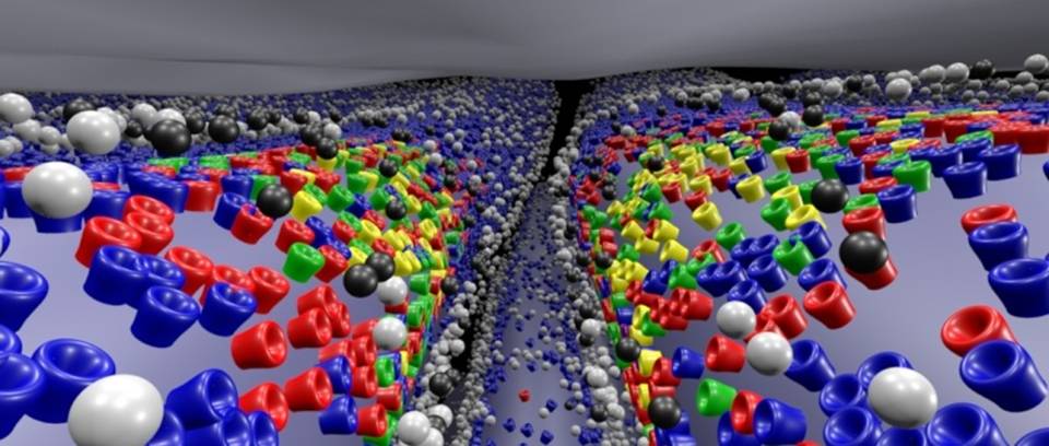
Figure 2. An
example showing the placement of the molecules (AchR and AchE) in NMJ
(from http://www.mcell.cnl.salk.edu)
1. Geometric Model
·
Mesh
model of neuro-muscular junction: We shall use the mesh model of a part of the
neuro-muscular junction provided by Dr. Tom Bartol of SALK Inst. The
visualization of the mesh can be seen in Figure 1. The mesh can be
downloaded from http://cvcweb.ices.utexas.edu/ccv/meshing/NMJ. The
lower contorted surface is of cell membrane and the volume enclosed by the two
is the synaptic cleft.
·
Molecules: There
are two sets of molecules we need to deal with in this modeling exercise. First
set consists of the AchR molecules (PDBID 2BG9) and the second set consists of
AchE (PDBID 1C2B).
The goal is to
1.
Devise an
automatic way of placing the AchR molecules in the thickened surface of the
cell membrane. The parameters are the densities of these molecules and their orientations
which might differ from molecule to molecule.
2.
Devise an
automatic way of placing the AchE molecules in the synaptic cleft. Again, the
parameters guide the density and orientations of these molecules.
In the next section we list some of the detailed
steps and the routines/algorithms that one might want to use/design to create
the spatially realistic model of a neuro-muscular junction.
2. Algorithms and Software
One possible way to populate the molecules in
their respective regions is to use the following (high-level) sketch. We
identify different modules that one needs to develop to accomplish the goal.
There could be variants of each step and ofcourse one might possibly think of a
completely different way to do the task. Therefore the following guideline is
rather indicative of a possible algorithm with necessary components than a lab
instruction manual.
1. Signed Distance Function
representation of Geometry
Given the mesh of neuro-muscular junction,
create a grid volume enclosing the mesh where every grid vertex has a scalar
value that denotes its distance from the mesh. The function sampled at these
vertices is the distance function. One can add a sign with the function value
where ![]() indicates that the
point is outside the volume enclosed by the mesh and
indicates that the
point is outside the volume enclosed by the mesh and ![]() indicates that it is
inside.
indicates that it is
inside.
While this produces a volume representation of
the mesh, from which the mesh can be re-extracted as the ![]() -set by any available contouring method, this doesn’t quite
serve the purpose for the geometry of the molecules obtained from Protein Data
Bank. There the geometry is a schematic representation of the atoms and bonds
in between. To convert them into signed distance volume one needs to do an
extra step of blurring the molecule using Gaussian kernel and take the level
set which produces a smooth approximation of the molecule. From the meshed
level set again one can use the SDF library to generate a volume of signed
distance function.
-set by any available contouring method, this doesn’t quite
serve the purpose for the geometry of the molecules obtained from Protein Data
Bank. There the geometry is a schematic representation of the atoms and bonds
in between. To convert them into signed distance volume one needs to do an
extra step of blurring the molecule using Gaussian kernel and take the level
set which produces a smooth approximation of the molecule. From the meshed
level set again one can use the SDF library to generate a volume of signed
distance function.
1. Routines
·
Blur: Use Exercise 1.
·
SDF: The library is called SDF Lib and it
can be downloaded from
http://cvcweb.ices.utexas.edu/ccv/usefulLinks.php.
2. Thickening of Cell Membrane
Once the SDF volume of the cell membrane is created
it is possible to obtain a thickness of the cell membrane geometry by taking an
interval volume in the grid where one isovalue corresponds to the membrane
geometry and the other isovalue produces a level set offset by a parameter from
the membrane surface. The interval volume therefore corresponds to a thickness
around the membrane surface. The second parameter of the interval volume guides
the amount of thickness.
1. Routines
LBIE-Mesher produces an interval volume from a
scalar volume.
3. Molecule Placement
In the above two steps we have created a
suitable computer representation of the platform where the placement procedure
can start. This process has two distinct parts - one for the placement of AchR
in the thickened membrane and the other for the placement of AchE in the
synaptic cleft. However the algorithm used is same and therefore we list that
only under a single subsection.
Placement of a single molecule is guided by a
set of parameters - Rotational and Positional. Following this set of parameters
one can orient the small SDF cube (volume) of a molecule. Now the task is to
penetrate the target volume and actually place it which requires a modification
in the SDF volume of the neuro-muscular junction to correctly reflect the
presence of the molecule so that if one performs a contouring of the level set
one gets the isosurface which indicates the protruding molecule at the desired
position and with the desired orientation.

Figure 3. From
left to right: AchR molecule, its placement parameters (intra-extra cellular
extents in the cell membrane) and one example embedding.
Once the placement of one molecule is achieved,
the process can be repeated to place the whole set where the density is guided
by another parameter. The paremeters required to place the molecules (AchR,
AchE) are described below. These parameters are crucial to obtain a spatially
realistic model of the whole system. So do read them carefully. More details
can be found in [4](Section 4.5, page 117).
·
Orientation
of AchR: The AchR molecules should be oriented in such
a way that they are normal to the surface of the cell membrane. As can be seen
from Figure 3 these molecules are elongated in one direction and that
direction should be perpendicular to the membrane surface. The intra/extra
cellular extent is also shown in Figure 3.
·
Density
of AchR: There are total 91,000 AchR to be placed on
the membrane surface. The density of AchR is not same though on different parts
of the membrane geometry. We divide the geometry into two parts - top
and middle. On the top part there will be total of 66,000
molecules and in the gorge (middle)there are total 25,000 molecules.

Figure 4. Basal
Lamina: A permeable membrane near the cell membrane where the tetrameric units
of AchE are to be placed. Right top figure shows a schematic diagram of one
such tetrameric unit. It has a tail which punctures the cell membrane and goes
inside. Right bottom figure shows a isosurface representation of the same color
coded according to electrostatic properties.
1.
Density
of AchE: The density of AchE is however same all
throughtout the basal lamina. There are total 59,000 AchE molecules distributed
in this region. The basal lamina is situated near the cell membrane surface.
For visualization, see Figure 4.
1. Routines
You need to devise an algorithm to do this
part. We list some high-level implementation ideas that one might follow.
Every voxel in the SDF volume of the
neuro-muscular junction can be flagged following their containment in the
boundary of the cell membrane, the thick interval volume around the cell
membrane surface, the basal lamina and the synaptic cleft. Create a
datastructure that holds the small SDF volume of a molecule along with its
other attributes, e.g. positional attributes etc. Each voxel then can have a
list of subvolumes for every molecule that is placed within the confinement of
that voxel. As we mentioned earlier, the function values at the vertices need
to be modified after each placement and this can be done locally.
4. Visualization: Level of Detail
Exploration
Although listed at the end of this sketch, this
part should be used to verify the correctness of your implementation in each
step. We encourage that you use TexMol for the visualization. It has a very
useful feature that will let you perform Level-of-Detail (LOD) visualization of
the model that you build. This part will have more details after Vinay and
Powei finishes incorporating their LOD viewer into TexMol.
5. Useful Tools and Libraries
You are encouraged to use some or all of the
tools and libraries listed here for this project. These tools are all available
from CCV Useful Links page. This list will be updated as we identify
some more tools and routines available that can be useful in this process. Also
we will give you more references to learn the functionalities and working
principle of these tools in detail.
·
SDF Lib
·
Blurrng
routine [1]
·
VolRover
·
TexMol [1]
·
LBIE-Mesher [5,6]
·
Contour
Spectrum [3]
·
Fast
Isocontour [2]
3. Milestones
In this project you are encouraged to use two
categories of software tools available at CVC - 1. Authoring software
that includes the modeling tools like TexMol, VolRover and Maya, 2. Player
software that includes Perfly, Interactive VolVideo (IVV) for interactive
display. For the scheduled timeline please see Table 1.
|
Oct 26 |
Project release, Discussion, Role
assignments |
|
Nov 2 |
Initial Models (Molecules + Membrane) |
|
|
Authoring + Player Software |
|
Nov 9 |
First unified model of NMJ |
|
|
Outline of further steps |
|
Nov 16 |
LOD (Level-of-detail) model of NMJ |
|
Nov 23 |
|
|
Nov 30 |
Augmenting models with properties
(Electrostatics, Hydrophobicity) |
|
|
Use of 3D textures |
|
Dec 7 |
Demo Day!!!
|
Table 1.
Timeline
References
[1] C.
Bajaj and P. Djeu and V. Siddavanahalli and A. Thane. Interactive Visual
Exploration of Large Flexible Multi-component Molecular Complexes. Proc. of
the Annual IEEE Visualization Conference, October 2004,
[2] C.
Bajaj and V. Pascucci and D. Schikore. Fast Isocontouring for Improved
Interactivity. Proceedings: ACM Siggraph/IEEE Symposium on Volume
Visualization, ACM Press, (1996),
[3] C.
Bajaj and V.Pascucci and D.Schikore. The Contour Spectrum. Proceedings of
the 1997 IEEE Visualization Conference, October 1997
[4] J.
R. Stiles and T. M. Bartol.
[5] Y.
Zhang and C. Bajaj. Adaptive and Quality Quadrilateral/Hexahedral Meshing from
Volumetric Data. In Computer Methods in Applied Mechanics and Engineering
(CMAME), in press, 2005.
[6] Y.
Zhang and C. Bajaj and B-S. Sohn. 3D Finite Element Meshing from Imaging Data.
In The special issue of Computer Methods in Applied Mechanics and
Engineering (CMAME) on Unstructured Mesh Generation, 194(48-49), pp.
5083-5106, 2005.
4. Project Participants
|
Name |
Team Assignment |
Description (currently empty) |
|
Bill Robins |
A-mol |
- |
|
Rick Bolkey |
A-mol |
- |
|
Shaolie Hossain |
A-mem |
- |
|
Albert Chen |
A-prop |
- |
|
Pai-Chi Li |
A-prop |
- |
|
Vinay Siddavanahalli |
A-mol |
- |
|
|
A-mem |
- |
|
Bongjune Kwon |
P |
- |
|
Jose Rivera |
P |
- |
|
Zeyun Yu |
A-mem |
- |
|
Jianguang Sun |
P |
- |
|
Katherine Clarridge |
? |
- |
|
Fred Nugen |
A-mem |
- |
|
Powei F |
P |
- |
|
Wenqi Zhao |
A-prop |
- |
|
Jessica Zhang |
A-prop |
- |
|
Samrat Goswami |
All |
- |
Table 2. Team
abbreviations: A-mol - Authoring software
(Molecule modeling), A-mem - Authoring software
(Membrane modeling), A-prop - Authoring software
(Properties), P - Player software.
The teams and their members:
·
Authoring
Software:
-
Molecule
team: Bill Robins, Rick Bolkey, Vinay.
-
Membrane
team: Shaolie Hossain, Fred Nugen,
-
Properties
team: Albert Chen, Wenqi Zhao, Jessica Zhang,
Pai-Chi Li.
·
Player
Software: Jianguang (Jason) Sun, Bongjune Kwon, Jose
Rivera, Powei Feng.
5. Progress and Guideline
1. Membrane Group
On Friday, Nov. 4th, the group submitted the
following requirement document.
Requirement document from Membrane group
Feedback from Dr. Bajaj on 5th Nov.,
2005
Revised requirement document from the
group on 8th Nov., 2005
2. Mol Group
On Friday, Nov. 4th, the group submitted the
following requirement document.
Requirement document from Mol group
Feedback from Dr. Bajaj on 5th Nov., 2005
Response from the group on 8th Nov.,
2005
3. Prop Group
On Friday, Nov. 4th, the group submitted the
following requirement document.
Requirement document from Prop group
Feedback from Dr. Bajaj on 5th Nov., 2005
Revised requirement document from the
group on 8th Nov., 2005
4. Player Group
On Friday, Nov. 4th, the group submitted the
following requirement document.
Requirement document from Player group
Feedback from Dr. Bajaj on 5th Nov., 2005
Revised
requirement document from the group on 8th Nov., 2005
6. Useful Links
The
document on how to use SGE to submit a job on prisms cluster is available on
prisms web page http://cvcweb.ices.utexas.edu/hardware/prismscluster/,
especially there is a tutorial on how to submit APBS jobs through SGE:
http://cvcweb.ices.utexas.edu/hardware/prismscluster/apbs.html