Subsection 2.3.6 Best rank-k approximation
¶We are now ready to answer the question "How do we find the best rank-k approximation for a picture (or, more generally, a matrix)? " posed in Subsection 2.1.1.
Theorem 2.3.6.1.
Given \(A \in \C^{m \times n}\text{,}\) let \(A = U \Sigma V^H \) be its SVD. Assume the entries on the main diagonal of \(\Sigma \) are \(\sigma_0 , \cdots , \sigma_{\min(m,n)-1} \) with \(\sigma_0 \geq \cdots \geq \sigma_{\min(m,n)-1} \geq 0 \text{.}\) Given \(k \) such that \(0 \leq k \leq min( m,n ) \text{,}\) partition
where \(U_L \in \C^{m \times k} \text{,}\) \(V_L \in \C^{n \times k} \text{,}\) and \(\Sigma_{TL} \in \R^{k \times k} \text{.}\) Then
is the matrix in \(\C^{m \times n} \) closest to \(A \) in the following sense:
In other words, \(B \) is the matrix with rank at most \(k \) that is closest to \(A \) as measured by the 2-norm. Also, for this \(B \text{,}\)
The proof of this theorem builds on the following insight:
Homework 2.3.6.1.
Given \(A \in \C^{m \times n}\text{,}\) let \(A = U \Sigma V^H \) be its SVD. Show that
where \(u_j \) and \(v_j \) equal the columns of \(U\) and \(V \) indexed by \(j \text{,}\) and \(\sigma_j \) equals the diagonal element of \(\Sigma\) indexed with \(j \text{.}\)
W.l.o.g. assume \(n \leq m \text{.}\) Rewrite \(A = U \Sigma V^H \) as \(A V = U \Sigma \text{.}\) Then
Hence \(A v_j = \sigma_j u_j \) for \(0 \leq j \lt n \text{.}\)
Proof of Theorem 2.3.6.1.
First, if \(B \) is as defined, then \(\| A - B \|_2 = \sigma_{k} \text{:}\)
(Obviously, this needs to be tidied up for the case where \(k \gt \rank( A ) \text{.}\))
Next, assume that \(C \) has rank \(r \leq k \) and \(\| A - C \|_2 \lt \| A - B \|_2 \text{.}\) We will show that this leads to a contradiction.
The null space of \(C \) has dimension at least \(n - k \) since \(\dim( \Null( C ) ) = n - r \text{.}\)
-
If \(x \in \Null( C ) \) then
\begin{equation*} \| A x \|_2 = \| ( A - C ) x \|_2 \leq \| A - C \|_2 \| x \|_2 \lt \sigma_{k} \| x \|_2. \end{equation*} Partition \(U = \left( \begin{array}{c | c | c} u_0 \amp \cdots \amp u_{m-1} \end{array} \right) \) and \(V = \left( \begin{array}{c | c | c} v_0 \amp \cdots \amp v_{n-1} \end{array} \right) \text{.}\) Then \(\| A v_j \|_2 = \| \sigma_j u_j \|_2 = \sigma_j \geq \sigma_{k} \) for \(j = 0, \ldots, k \text{.}\)
-
Now, let \(y \) be any linear combination of \(v_0, \ldots, v_k \text{:}\) \(y = \alpha_0 v_0 + \cdots + \alpha_k v_k \text{.}\) Notice that
\begin{equation*} \| y \|_2^2 = \| \alpha_0 v_0 + \cdots + \alpha_k v_k \|_2^2 = \vert \alpha_0 \vert^2 + \cdots \vert \alpha_k \vert^2 \end{equation*}since the vectors \(v_j \) are orthonormal. Then
\begin{equation*} \begin{array}{l} \| A y \|_2^2 \\ ~~~=~~~~ \lt y =\alpha_0 v_0 + \cdots + \alpha_k v_k \gt \\ \| A ( \alpha_0 v_0 + \cdots + \alpha_k v_k ) \|_2^2 \\ ~~~=~~~~ \lt {\rm distributivity} \gt \\ \| \alpha_0 A v_0 + \cdots + \alpha_k A v_k \|_2^2 \\ ~~~=~~~~ \lt A v_j = \sigma_j u_j \gt \\ \| \alpha_0 \sigma_0 u_0 + \cdots + \alpha_k \sigma_k u_k \|_2^2 \\ ~~~= ~~~~\lt \mbox{ this works because the } u_j \mbox{ are orthonormal } \gt \\ \| \alpha_0 \sigma_0 u_0 \|_2^2 + \cdots + \| \alpha_k \sigma_k u_k \|_2^2 \\ ~~~=~~~~ \lt \mbox{ norms are homogeneous and } \| u_j \|_2 = 1 \gt \\ \vert \alpha_0 \vert^2 \sigma_0^2 + \cdots + \vert \alpha_k \vert^2 \sigma_k^2 \\ ~~~ \geq ~~~~ \lt \sigma_0 \geq \sigma_1 \geq \cdots \geq \sigma_k \geq 0 \gt \\ ( \vert \alpha_0 \vert^2 + \cdots + \vert \alpha_k \vert^2 ) \sigma_k^2 \\ ~~~ = ~~~~ \lt \| y \|_2^2 = \vert \alpha_0 \vert^2 + \cdots + \vert \alpha_k \vert^2 \gt \\ \sigma_k^2 \| y \|_2^2. \end{array} \end{equation*}so that \(\| A y \|_2 \geq \sigma_k \| y \|_2 \text{.}\) In other words, vectors in the subspace of all linear combinations of \(\{ v_0, \ldots , v_k \} \) satisfy \(\| A x \|_2 \geq \sigma_k \| x \|_2 \text{.}\) The dimension of this subspace is \(k+1 \) (since \(\{ v_0, \cdots , v_{k} \} \) form an orthonormal basis).
Both these subspaces are subspaces of \(\Cn \text{.}\) One has dimension \(k+ 1 \) and the other \(n - k \text{.}\) This means that if you take a basis for one (which consists of \(n-k \) linearly independent vectors) and add it to a basis for the other (which has \(k + 1 \) linearly independent vectors), you end up with \(n + 1\) vectors. Since these cannot all be linearly independent in \(\Cn \text{,}\) there must be at least one nonzero vector \(z \) that satisfies both \(\| A z \|_2 \lt \sigma_k \| z \|_2 \) and \(\| A z \|_2 \geq \sigma_k \| z \|_2 \text{,}\) which is a contradiction.
Theorem 2.3.6.1 tells us how to pick the best approximation to a given matrix of a given desired rank. In Section Subsection 2.1.1 we discussed how a low rank matrix can be used to compress data. The SVD thus gives the best such rank-k approximation. Let us revisit this.
Let \(A \in \Rmxn \) be a matrix that, for example, stores a picture. In this case, the \(i,j\) entry in \(A \) is, for example, a number that represents the grayscale value of pixel \((i,j) \text{.}\)
Homework 2.3.6.2.
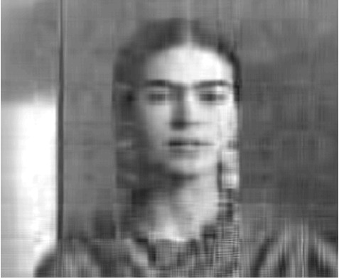
In Assignments/Week02/matlab execute
IMG = imread( 'Frida.jpg' );
A = double( IMG( :,:,1 ) );
imshow( uint8( A ) )
size( A )
to generate the picture of Mexican artist Frida Kahlo

Although the picture is black and white, it was read as if it is a color image, which means a \(m \times n \times 3 \) array of pixel information is stored. Setting A = IMG( :,:,1 ) extracts a single matrix of pixel information. (If you start with a color picture, you will want to approximate IMG( :,:,1), IMG( :,:,2), and IMG( :,:,3) separately.)
Next, compute the SVD of matrix \(A \)
[ U, Sigma, V ] = svd( A );
and approximate the picture with a rank-k update, starting with \(k = 1 \text{:}\)
k = 1
B = uint8( U( :, 1:k ) * Sigma( 1:k,1:k ) * V( :, 1:k )' );
imshow( B );

Repeat this with increasing \(k \text{.}\)
r = min( size( A ) )
for k=1:r
   imshow( uint8( U( :, 1:k ) * Sigma( 1:k,1:k ) * V( :, 1:k )' ) );
   input( strcat( num2str( k ), "    press return" ) );
end
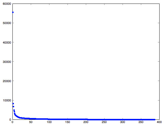
To determine a reasonable value for \(k \text{,}\) it helps to graph the singular values:
figure
r = min( size( A )  );
plot( [ 1:r ], diag( Sigma ), 'x' );
Since the singular values span a broad range, we may want to plot them with a log-log plot
loglog( [ 1:r ], diag( Sigma ), 'x' );
For this particular matrix (picture), there is no dramatic drop in the singular values that makes it obvious what \(k \) is a natural choice.
k = 1
\(k = 2 \)

\(k=5 \)
\(k = 10 \)
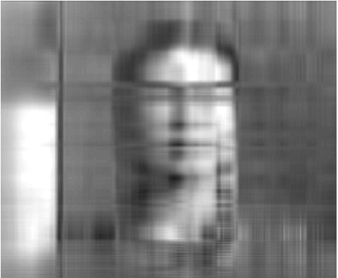
\(k=25 \)
Original picture