Subsection 2.3.3 An "algorithm" for computing the SVD
¶We really should have created a video for this section. Those who have taken our "Programming for Correctness" course will recognize what we are trying to describe here. Regardless, you can safely skip this unit without permanent (or even temporary) damage to your linear algebra understanding.
In this unit, we show how the insights from the last unit can be molded into an "algorithm" for computing the SVD. We put algorithm in quotes because while the details of the algorithm mathematically exist, they are actually very difficult to compute in practice. So, this is not a practical algorithm. We will not discuss a practical algorithm until the very end of the course, in Week 11.
We observed that, starting with matrix \(A \text{,}\) we can compute one step towards the SVD. If we overwrite \(A \) with the intermediate results, this means that after one step
where \(\widehat A \) allows us to refer to the original contents of \(A \text{.}\)
In our proof of Theorem 2.3.1.1, we then said that the SVD of \(B \text{,}\) \(B = U_B \Sigma_B V_B^H \) could be computed, and the desired \(U\) and \(V \) can then be created by computing \(U = \widetilde U U_B \) and \(V = \widetilde V V_B \text{.}\)
Alternatively, one can accumulate \(U \) and \(V \) every time a new singular value is exposed. In this approach, you start by setting \(U = I_{m \times m}\) and \(V = I_{n \times n} \text{.}\) Upon completing the first step (which computes the first singular value), one multiplies \(U \) and \(V \) from the right with the computed \(\widetilde U \) and \(\widetilde V \text{:}\)
Now, every time another singular value is computed in future steps, the corresponding unitary matrices are similarly accumulated into \(U \) and \(V \text{.}\)
To explain this more completely, assume that the process has proceeded for \(k \) steps to the point where
where the current contents of \(A \) are
This means that in the current step we need to update the contents of \(A_{BR} \) with
and update
which simplify to
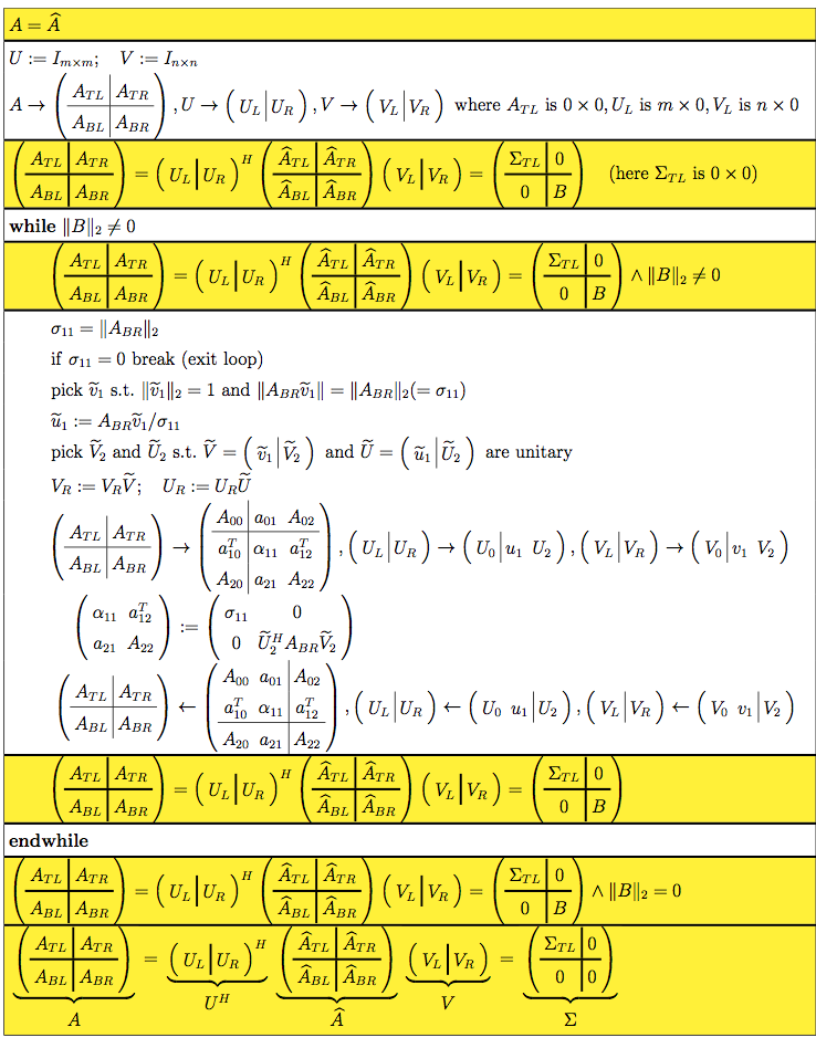
At that point, \(A_{TL} \) is expanded by one row and column, and the left-most columns of \(U_R \) and \(V_R\) are moved to \(U_L \) and \(V_L \text{,}\) respectively. If \(A_{BR} \) ever contains a zero matrix, the process completes with \(A \) overwritten with \(\Sigma = U^H \widehat V \text{.}\) These observations, with all details, are captured in Figure 2.3.3.1. In that figure, the boxes in yellow are assertions that capture the current contents of the variables. Those familiar with proving loops correct will recognize the first and last such box as the precondition and postcondition for the operation and
as the loop-invariant that can be used to prove the correctness of the loop via a proof by induction.
The reason this algorithm is not practical is that many of the steps are easy to state mathematically, but difficult (computationally expensive) to compute in practice. In particular:
Computing \(\| A_{BR} \|_2 \) is tricky and as a result, so is computing \(\widetilde v_1 \text{.}\)
Given a vector, determining a unitary matrix with that vector as its first column is computationally expensive.
Assuming for simplicity that \(m = n \text{,}\) even if all other computations were free, computing the product \(A_{22} := \widetilde U_2^H A_{BR} \widetilde V_2\) requires \(O( (m-k)^3 ) \) operations. This means that the entire algorithm requires \(O( m^4 ) \) computations, which is prohibitively expensive when \(n \) gets large. (We will see that most practical algorithms discussed in this course cost \(O( m^3 ) \) operations or less.)
Later in this course, we will discuss an algorithm that has an effective cost of \(O( m^3 ) \) (when \(m = n \)).
Ponder This 2.3.3.1.
An implementation of the "algorithm" in Figure 2.3.3.1, using our FLAME API for Matlab (FLAME@lab) [5] that allows the code to closely resemble the algorithm as we present it, is given in mySVD.m (Assignments/Week02/matlab/mySVD.m). This implemention depends on routines in subdirectory Assignments/flameatlab being in the path. Examine this code. What do you notice? Execute it with
m = 5;
n = 4;
A = rand( m, n );      % create m x n random matrix
[ U, Sigma, V ] = mySVD( A )
Then check whether the resulting matrices form the SVD:
norm( A - U * Sigma * V' )and whether \(U \) and \(V \) are unitary
norm( eye( n,n ) - V' * V )
norm( eye( m,m ) - U' * U )