CS/CAM/BME 395T - #54303
Multi-scale Bio-Modeling and Visualization
Exercise 1: ----------- Molecular modeling I – Constructing and
visualizing computer models from the PDB, VIPER,
TexMol (http://ccvweb.csres.utexas.edu/ccv/projects/project.php?proID=8) is a program developed at CVC and includes molecule visualization, electron density/hydrophobicity computations, surface computations and other useful functions. VolRover (http://ccvweb.csres.utexas.edu/ccv/projects/project.php?pageIndex=1&proID=9) is another tool to look at large volume datasets.
In this exercise, you can learn:
- The structure of simple proteins and RNA
- How to express (approximate) electron density as a sum of Gaussians.
- Simple file formats including the well known .pdb ( for atoms ) and our own .rawiv, .rawv ( volume ) and .raw ( surface ) file formats.
- Rendering: geometry and volume rendering.
Running TexMol
Lab machines:
In the Graphic Lab (ACES 2nd floor: CS Lab 2.102), there are Windows and Linux machines, all with the latest version of TexMol installed in it. Please ask Jason Sun (jgsun@ices.utexas.edu) and Dr Bajaj (bajaj@cs.utexas.edu) for accounts if you do not have any. Email Vinay (skvinay@cs.utexas.edu) on issues with running TexMol.
Installing on other machines:
Download TexMol (from www.ices.utexas.edu/cvc) and install it. It needs QT (www.trolltech.com) and Cg (from NVidia) to work. You will also need to install OpenGL. If you installed TexMol, VolRover is easy to install. It should run on both Windows and Linux OS. If you do not have an NVidia FX or above, the rendering may not work properly. For this class, we also provide binaries of TexMol on cvc's software download page: http://ccvweb.csres.utexas.edu/ccv/projects/project.php?proID=8 or http://ccvweb.csres.utexas.edu/software/.
Homework:
- Download hemoglobin
(1A00.pdb) from www.pdb.org and load into TexMol. Make images of the union
of spheres model with atom colors + residue colors + chain colors separately.
Construct the electron density (utilities -> construct volume) and
volume render the function. Play around with the transfer function control
widget at the bottom and make an image of the volume. Add an isocontour
(with isovalue 1: check the mouse tip by moving the mouse over the
isocontour bar) and make another image after removing the volume rendering
by making the volume transparent in the transfer function. Construct the
molecular surface by using the utilities -> construct surface menu item
and make another image. All images should be of the same view point.
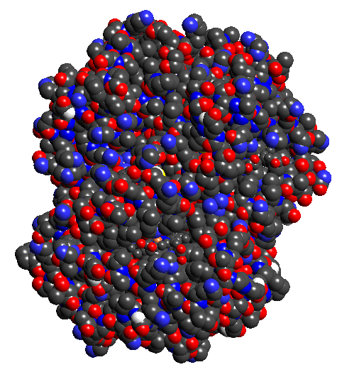
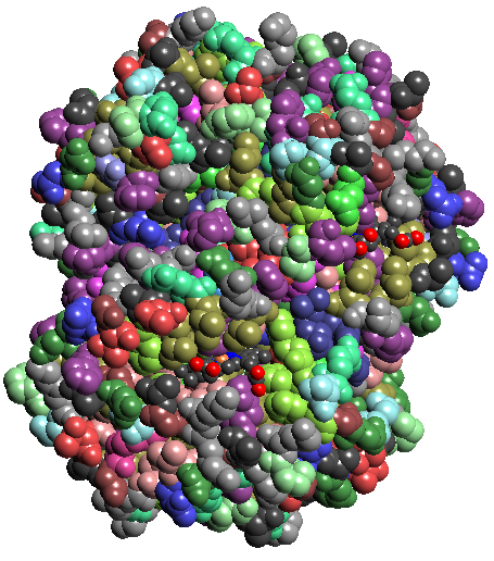
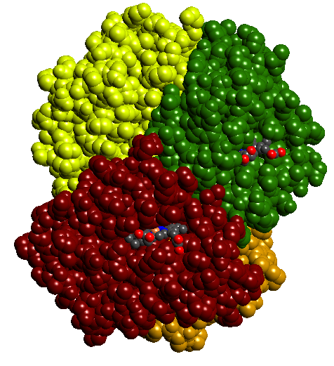
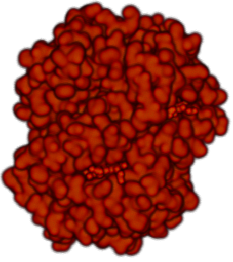
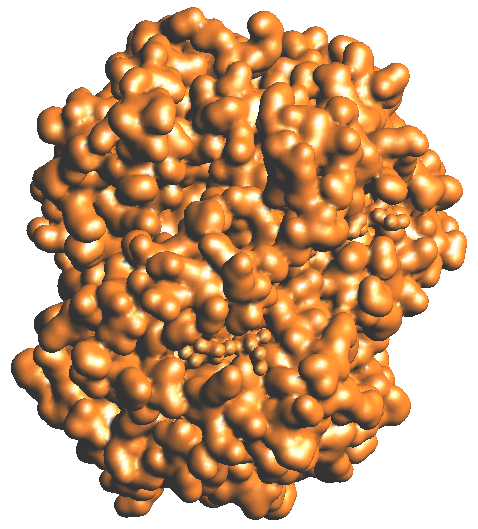
1a: atomic colors 1b: residue colors 1c: chain colors 1d: Gaussian blur vol rendering 1e:Isocontour of Gaussian blurring
Figure 1: Hemoglobin (1A00.pdb)
- For the list of viruses
assigned to you (from the table below, see an accompanying file for the
assignments), create RawV volume files
and images. If it is an icosahedral virus, and the atomic coordinates are
present in the Viper website, use that. Otherwise, download from the PDB
website. Please delete all HETATMs from the files. (Open pdb or pdb1 file
in an ascii text editor, delete all lines that begin with a HETATM)
Creating volume files: Use TexMol in the command prompt:
- Using a colormap file:
use: <TexMol exe> -blur <input atomic file> <output RawV file> <dim1> <dim2> <dim3> 0 true <Gaussian rate of decay> 0 <colormap file> 0 0 1
Color map: See colormapRawV.htm for the colormap documentation. Be creative in using different colors.
- Define the SAS, SES, VDW
surfaces. Define the Gaussian based approximation to the SES. Express the
surface as an isocontour of the convolution of Gaussians, including the
rate of decay and van der Waals radii as parameters.
- An alternative to asking the
user to input the rate of decay of the Gaussian is to ask for a
'resolution' parameter. Here is one definition (This definition is shaky
and unclear.): The resolution is equal to half the width of a Gaussian in
Angstroms, where the Gaussian multiplied by a function of the radius of
the atom. How would you approximate the previous definition of the
Gaussian (which includes the rate of decay and radii) to the new one
(which includes only the resolution and radii) ?
- Familiarize yourself with the
two websites: PDB website (http://www.rcsb.org/pdb) Viper website (http://mmtsb.scripps.edu/viper/).
- Write a couple of statements
defining 'docking' of molecules. Download any complex (2 or more proteins
complexed together) from www.pdb.org. Break it up into 2 separate pdb
files. Visualize, at the same time, one protein with atom colors and
another with residue colors to see the complex and the two individual components
in it.
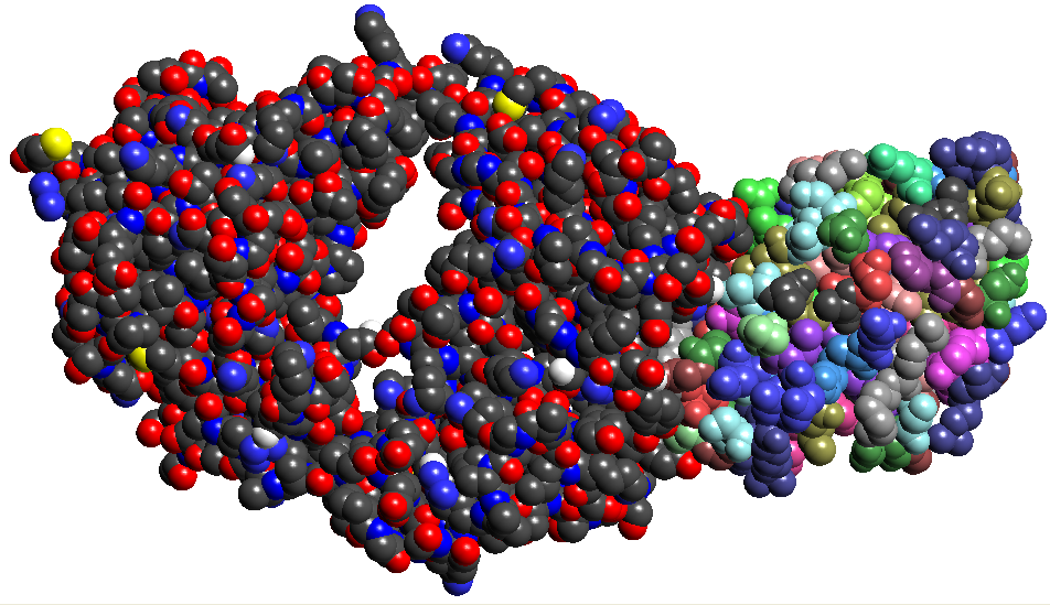
Figure 6: Antibody Antigen complex of 1BQL.PDB. The Fab chains are on the left in atomic colors and the Lysozyme on the right with residue colors
|
|
Color map
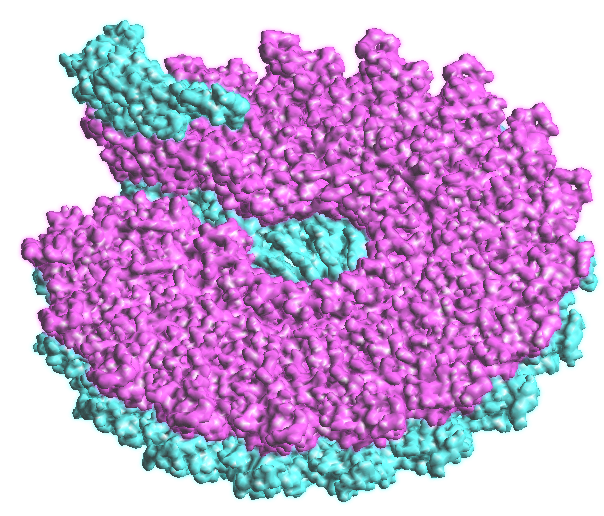
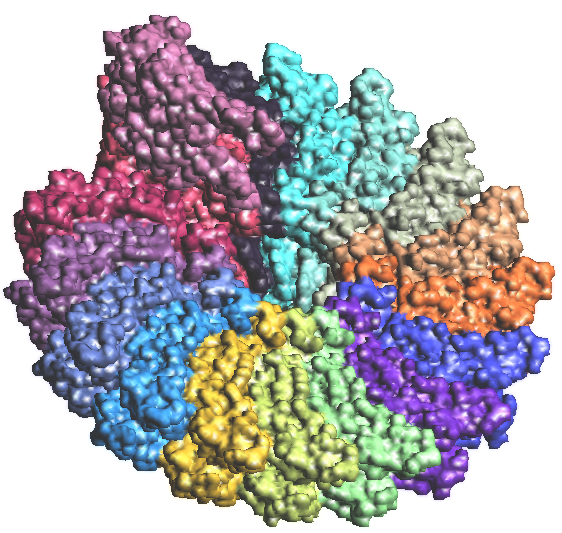
used: --------------------../Dataset/1EI7_chains.cmap------------------------------ # TMV COAT PROTEIN REFINED FROM THE 4-LAYER
AGGREGATE -------------------------------------------------------------------------------- Command: moleculeviz -blur ../dataset/1EI7.pdb ../dataset/1EI7_chain_color.rawv 128 128 128 0 true -2.3 0 ../Dataset/1EI7_chains.cmap 0 0 1 |
|
Figure 2a: TMV coat protein 1EI7.PDB |
|
|
|
Color map
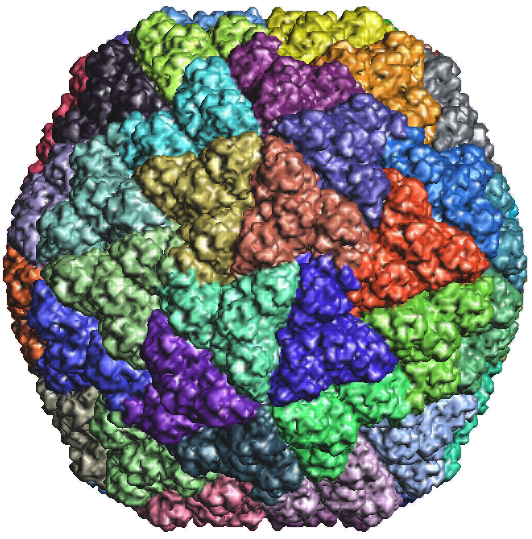
used: --------------------../Dataset/1uf2_chains.cmap------------------------------ # the following line is implied but included as
an example -------------------------------------------------------------------------------- Command: moleculeviz -blur ../dataset/1uf2.pdb1 ../dataset/1uf2_chains.rawv 128 128 128 0 true -2.3 0 ../Dataset/1uf2_chains.cmap 0 0 1 |
|
Figure 2b: Rice Dwarf Virus capsid 1UF2.PDB1 |
|
- Using color by capsomer:
use: (for pdb1 files) <TexMol exe> -blur
<input atomic file> <output RawV file> <dim1> <dim2>
<dim3> 0 true <Gaussian rate of decay> 4 "" 0 0 1
use: (for pdb files) <TexMol exe> -blur
<input atomic file> <output RawV file> <dim1> <dim2>
<dim3> 0 true <Gaussian rate of decay> 1 "" 0 0 1
|
|
Command: moleculeviz -blur ../dataset/1EI7.pdb ../dataset/1EI7_capsomer_color.rawv 128 128 128 0 true -2.3 4 "" 0 0 1 |
|
Figure 2c: TMV coat protein 1EI7.PDB |
|
|
|
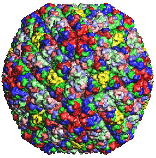
Command: moleculeviz -blur ../dataset/1uf2.pdb1
../dataset/1uf2_color.rawv 128 128 128 0 true -2.3 4 "" 0 0 1
|
|
Figure 2d: Rice Dwarf Virus outer capsid 1UF2.PDB1 |
|
Make an image of the volume rendering of the blurred virus
(the created .RawV file, by loading it into TexMol), add an isocontour, save the isocontour as a rawnc
file, load it separately and make another image.
Write a short (2-3lines) description of the molecule, including its PDB
id, the size in atoms, size in dimensions of volume, rate of decay used,
captions for each image.
Since there will be a learning curve to the software and new file formats, feel free to contact Vinay. skvinay@cs.utexas.edu
Here is the assignment sheet
Turning in homework:
There are two parts to be submitted. First, the report which includes images and answers (no data files) should be sent to Dr Bajaj as a single pdf or html file. The volume RawV files for part 2, along with the description + images + image captions should be zipped and uploaded to any of your websites. If you do not have access to a webspace, please contact Jason (jgsun@ices.utexas.edu) for an alternative method to upload your results.
Table of virus models.
|
|
Name |
Family |
Host |
NA |
Capisd Sym.
(# T) |
#Shell
(E?) |
Modality
(res
in A) (pdbid) |
|
1 |
Tobacco mosaic |
Tobamoviridae |
P |
sR
(L) |
He |
1(n) |
X(2.45) (1ei7) |
|
|
Ebola |
Filoviridae |
V |
sR (L) |
He |
1(E) |
X(3) (1ebo) |
|
|
Vaccinia |
Poxviridae |
V |
dD (L) |
He |
1(E) |
X(1.8)
(1luz) |
|
|
Rabies |
Rhabdoviridae |
V |
sR(L) |
He |
1(E) |
X(1.5)
(1vyi) |
|
|
Satellite tobacco necrosis |
Tombusviridae |
P |
sR
(L) |
Ic (1) |
1(n) |
X(2.5) (2stv) |
|
|
L-A (Saccharomyces cerevisiae) |
Totiviridae |
F |
dR (L) |
Ic
(1) |
1(n) |
X(3.6) (1m1c) |
|
|
Canine parvovirus-Fab complex |
Parvoviridae |
V |
sD (L) |
Ic
(1) |
1(n) |
X(3.3) (2cas) |
|
|
T1L reovirus core |
Reoviridae |
V |
dR
(L) |
Ic
(1,1) |
2(n) |
X(3.6) (1ej6) |
|
|
T3D reovirus core |
Reoviridae |
V |
dR
(L) |
Ic
(1,1) |
2(n)
|
X(2.5)
(1muk) |
|
|
P4 (Ustilago maydis) |
Totiviridae |
P |
dR
(L) |
Ic
(1) |
1(n)
|
X(1.8)
(1kp6) |
|
|
Tomato bushy stunt |
Tombusviridae |
P |
sR (L) |
Ic
(3) |
1(n) |
X(2.9) (2tbv) |
|
|
Cowpea Chlorotic Mosaic |
Bromoviridae |
P |
sR
(L) |
Ic
(3) |
1(n)
|
X(3.2) (1cwp) |
|
|
Cucumber mosaic |
Bromoviridae |
P |
sR
(L) |
Ic
(3) |
1(n)
|
X(3.2) (1f15) |
|
|
|
Caliciviridae |
V |
sR
(L) |
Ic
(3) |
1(n)
|
X(3.4) (1ihm) |
|
|
Rabbit hemorrhagic disease VLP-MAb-E3 complex |
Caliciviridae |
V |
sR
(L) |
Ic
(3) |
1(n) |
X(2.5)
(1khv) |
|
|
Galleria mellonella denso |
Parvoviridae |
I |
sD (L) |
Ic
(1) |
1(n) |
X(3.7) (1dnv) |
|
|
|
Togaviridae |
I,V |
sR |
Ic
(4,1) |
2(E)
|
C(9)
(1dyl) |
|
|
Polyoma |
Papovaviridae |
V |
dD
(C) |
Ic
(7D) |
1(n) |
X(2.2)
(1cn3) |
|
|
Simian |
Papovaviridae |
V |
dD
(C) |
Ic
(7D) |
1(n)
|
X(3.1) (1sva) |
|
|
Papillomavirus Initiation Complex |
Papovaviridae |
V |
dD
(C) |
Ic
(7D) |
1(n) |
X(3.2)
(1ksx) |
|
|
Blue Tongue |
Reoviridae |
V |
dR
(L) |
Ic
(1,13L) |
2(n) |
X(3.5) (2btv) |
|
|
Rice dwarf |
Reoviridae |
P |
dR (L) |
Ic
(1,13L) |
2(n) |
X(3.5) (1uf2) |
|
|
T1L reovirus virion |
Reoviridae |
V |
dR
(L) |
Ic
(1,13L) |
2(n) |
X(2.8)
(1jmu) |
|
|
Simian rotavirus (SA11-4F) TLP |
Reoviridae |
V |
dR
(L) |
Ic
(1,13L) |
2(n) |
X(2.38)
(1lj2) |
|
|
Rhesus rotavirus |
Reoviridae |
V |
dR
(L) |
Ic
(1,13L) |
2(n) |
X(1.4)
(1kqr) |
|
|
Nudaurelia capensis w |
Tetraviridae |
I |
sR
(L) |
Ic
(4) |
1(n)
|
X(2.8)
(1ohf) |
|
|
Herpes Simplex |
Herpesviridae |
V |
dD
(L) |
Ic
(7L) |
1(E)
|
X(2.65)
(1jma) |
|
|
HepBc (human liver) (nHBc) |
Hepadnaviridae |
V |
dD
(C) |
Ic(4) |
1(E)
|
X(3.3) (1qgt) |
Table: Helical and Icosahedral Viruses: (2) Name of virus (3) Family nomencleature from the ICTV database (4) Host types are P for Plant, V for Vertebrate, I for Invertebrate, F for Fungi (5) Virus Nucleic Acid (NA) type is single stranded RNA (sR) or DNA (sD), double stranded RNA (dR) or DNA (dD) and linear (L) or circular (C) (6) Capsid symmetry is Helix (He) or Icosahedral (Ic) with the triangulation number of each capsid shell in parenthesis (7) The number of capsid shells and whether enveloped (E) or not (n) (8) The acquisition modality X-ray, feature resolution and PDB id in parenthesis.