Competing at the 2026 UChicago Trading Competition

A technical writeup of the models, execution logic, and lessons from Case 1.

April 14, 2026

This spring, our team from UT Austin was selected to compete in the 14th Annual UChicago Trading Competition, hosted by the University of Chicago Financial Markets Program at Convene Willis Tower in Chicago. The competition brings together students from across the country — this year over 150 participants from 31 universities — to compete in algorithmic trading across two cases.

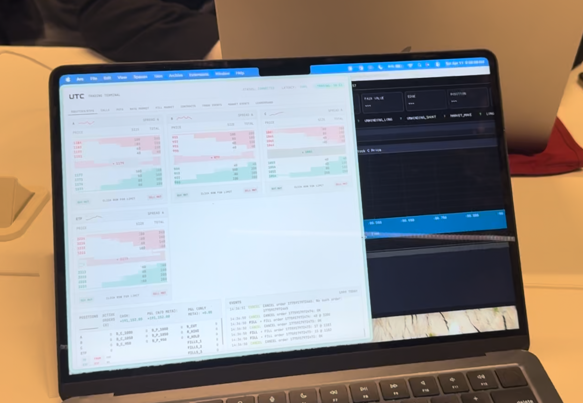
Case 1 was a live market making case run on X-Change, the Financial Markets Program's in-house exchange simulator. Teams write algorithms in Python and trade against each other and a set of exchange bots across twelve 15-minute rounds over three hours. Case 2 was a portfolio optimization case submitted before the competition.

This post focuses on Case 1, specifically the fair value model and execution logic we built for Stock C, which was my primary contribution.

What Is the UChicago Trading Competition?

The UTC is an annual algorithmic trading competition hosted by the University of Chicago's Financial Markets Program, supported by firms including Citadel, Jane Street, Optiver, IMC, SIG, and Old Mission Capital. It is one of the most intellectually demanding events in the quantitative finance space.

The competition has two cases:

• Case 1: Market Making — live algorithmic trading on the X-Change platform, run in real time on the day of the competition.
• Case 2: Portfolio Optimization — pre-submitted Python code evaluated on a 12-month out-of-sample period.

What We Were Trading

The instrument universe for Case 1 was deliberately complex:

• Stock A — driven by earnings releases and news headlines.
• Stock B — a semiconductor company with only option instruments.
• Stock C — a large-cap insurance company sensitive to earnings and interest rates.
• ETF — a basket of 1A + 1B + 1C.
• Fed Rate Prediction Markets — contracts on hike, hold, or cut rates.

Stock A: A Brief Overview

Stock A was primarily built by my teammate. The strategy utilized two distinct entry triggers:

1. Earnings Events: On each EPS release, the bot computes $FV = EPS \times PE$ (with $PE$ constant at 10). If the edge ($FV - mid$) is positive, it accumulates longs up to 200 shares in chunks of 40. To avoid noisy re-entries near parity, the bot only exits once the edge falls below a 2-unit buffer. Entries utilize aggressive limit prices — best_ask + 5 for buys, best_bid - 5 for sells — ensuring fast fills without walking the book into thin liquidity.

2. Sentiment Analysis: For unstructured news, we used a pre-catalogued lookup table of 80+ exact headlines mapped to signed sentiment weights. This allowed for directional positioning at market speed. Unknown headlines triggered an immediate exit to flat to minimize risk. Notably, every Stock A order was mirrored with an ETF order of the same size and direction, effectively doubling directional exposure on high-confidence signals.

The case packet provided the exact formulas for Stock C's fair value. The challenge was calibrating the parameters and building execution logic fast enough to trade on them live. Here's what that formula looks like:

Stock C: Building the Fair Value Model

I was responsible for developing the fair value model and execution logic for Stock C. It's the most mathematically involved instrument in the case — a large insurance company whose price is simultaneously sensitive to earnings, interest rates, and bond portfolio dynamics.

Step 1 — Extract Fed probabilities from prediction market mids

Normalize the three prediction market contracts to sum to 1:

Step 2 — Compute expected rate change and yield shift

Step 3 — Rate-adjusted P/E ratio

Step 4 — Bond portfolio value change (duration-convexity approximation)

The Taylor expansion captures both the first-order (duration) and second-order (convexity) effects of yield changes on bond prices:

In code, this runs on every prediction market book tick (implemented for Stock C):

def _compute_fv(self) -> Optional[tuple[float, float]]:
    total = self._m_hike + self._m_hold + self._m_cut
    q_hike = self._m_hike / total
    q_cut  = self._m_cut / total
    e_dr   = 25.0 * q_hike - 25.0 * q_cut
    dy     = BETA_Y * e_dr                       # BETA_Y = 0.000945
    pe_t   = PE_0 * math.exp(-GAMMA * dy)        # PE_0 = 14.0, GAMMA = 3.49
    ops    = self._eps * pe_t
    bond   = LAM * B0_N * (-D_DUR * dy + 0.5 * CONV * dy ** 2)
    fv     = ops + bond
    mid    = self.market_state.mid("C")
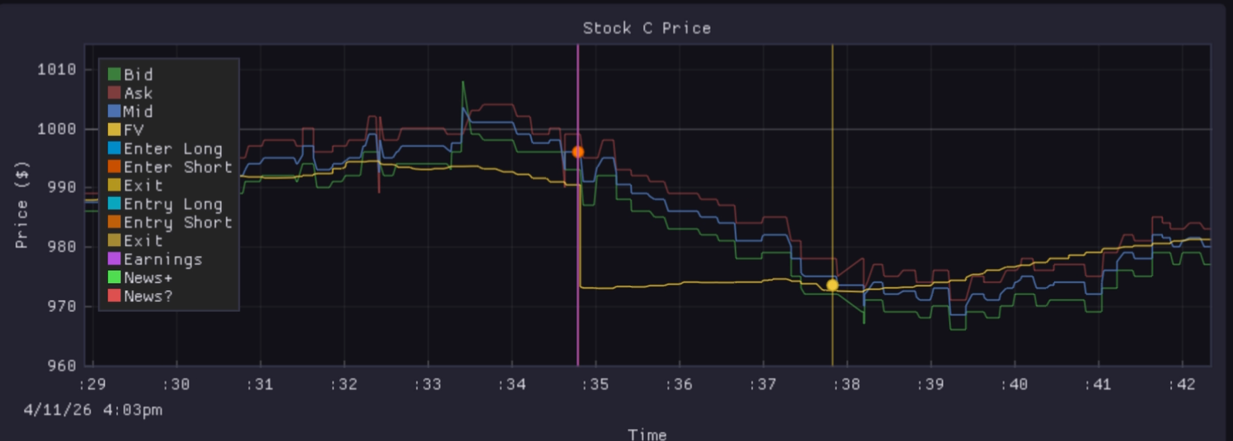
    return fv, fv - mid                          # (fair value, edge)

One additional layer on top of the model: CPI front-running. When a CPI print arrives as structured news, the bot immediately shifts the hike/cut probability mass before the prediction market has repriced. A positive surprise — actual CPI higher than forecast — shifts weight toward a hike, compressing the P/E and reducing bond value in the model before most other bots have reacted to the same data. This adjustment is stored as a persistent offset layered on top of the next market mid read:

def update_from_cpi(self, forecast: float, actual: float) -> None:
    surprise = actual - forecast
    adjustment = self.cpi_sensitivity * surprise
    self._cpi_adjustment = max(-0.3, min(0.3, adjustment))
    self._recompute()

The intent was simple: position before the crowd moves the book.

Stock C: The Trading Logic

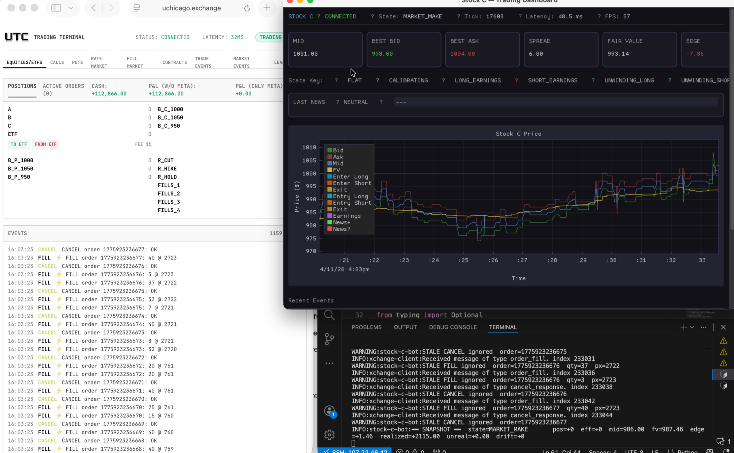
With a fair value in hand, the bot operates as a state machine with six states:

• FLAT — no position, waiting for a meaningful edge signal. The bot will not re-enter a position from this state until a new earnings or yield update fires. This prevents re-entry on stale fair values between events.
• LONG_EARNINGS — edge is positive (stock is cheap relative to FV). The bot is actively accumulating longs in chunks of 40, up to a maximum of 200 shares. Every book tick triggers another evaluate call, stacking orders until the position limit is hit or the edge reverses.
• SHORT_EARNINGS — mirror of the above. Edge is negative (stock is expensive). Bot accumulates shorts in the same chunked fashion down to −200.
• UNWINDING_LONG — the edge has crossed back toward zero. The bot cancels any remaining buy orders and submits chunked market sell orders to drive the position back to flat. No new directional orders are placed in this state.
• UNWINDING_SHORT — same as above, but buying to cover a short position.
• MARKET_MAKE — a post-unwind holding state. After a full unwind completes, the bot parks here rather than returning directly to FLAT. In practice this state was a placeholder during the competition — passive market making logic was built but not deployed in live rounds.

The EPS exit rule was the most important piece of execution logic. When new earnings arrive for Stock C, the bot:

• Immediately cancels all open orders.
• Sets a pending flag — the new EPS is not applied yet.
• On the very next book tick, closes any open position at the current market price.
• Then applies the new EPS and re-evaluates fair value.

async def _apply_eps_exit(self) -> None:
    self._eps_pending = False
    server_pos = self.positions.get("C", 0)
    if server_pos != 0:
        await self._cancel_all_orders()
        await self._close_position("C")          # close at PRE-repricing price
    if self._eps_pending_val is not None:
        self._eps = self._eps_pending_val        # NOW apply new EPS
        self._eps_pending_val = None
    self._state = BotState.FLAT
    self._long_short_eligible = True
    await self._request_evaluate()               # re-enter with new FV

The one-tick delay is deliberate. Without it, the bot is holding a position at a stale price exactly when the market is repricing — a classic "skunk stop." The pending flag pattern ensures the bot is always flat before the fair value jump, then re-enters cleanly based on the updated signal.

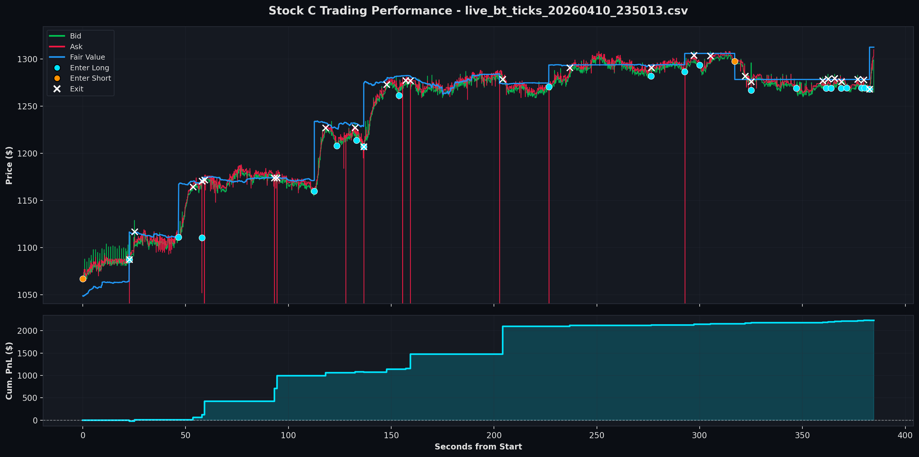
Results: Rounds 1–6

Through the first six rounds, the strategy worked cleanly. The OLS-calibrated parameters tracked market price discovery closely, and the CPI front-running added measurable alpha. We placed 1st overall through this stretch.

What Changed After Round 6

The transition wasn't a single event — it was gradual, and noticeable in the logs before it was obvious in the P&L. Bid-ask spreads on Stock C started widening. The size sitting at the top of the book shrank. Opposing bots began reacting to news faster, meaning the window between a CPI print arriving and the prediction market repricing — the window our CPI front-running relied on — compressed significantly.

A few things broke in combination:

• Market orders became expensive. In early rounds, sending a market buy for 40 shares filled near mid. In later rounds, with only 10–15 shares sitting at the best ask, a 40-share market order would consume the top level and fill the remainder at the next level up — paying a spread we hadn't accounted for when sizing the trade.
• Unwinding became costly. Closing a 200-share position via five sequential market orders in a thin book meant each chunk moved the market against us. By the time the fifth chunk filled, we were selling into a price we'd helped push down ourselves.
• The edge threshold didn't adapt. The bot entered positions when edge > 0 and exited when edge reversed — but in thin, noisy books, the mid price was jumping around more than in early rounds. A genuine edge of +2 looked the same as noise of +2, and the fixed threshold couldn't distinguish between them.

The core fair value model remained accurate throughout. The parameters didn't drift and the formula continued to track the market's price discovery closely. The problem was entirely on the execution side — a model problem and an execution problem are very different things, and in rounds 6–12 we were fighting the latter.

Takeaways

• Signal vs. Execution: The FV model was robust, but execution degraded in thin later-round books, highlighting the need for dynamic order sizing.
• Preparation: Pre-calibrating parameters using OLS on historical data yielded an R² of 0.934, providing confidence from the first tick.
• Observability: Building a real-time dashboard allowed us to diagnose and fix issues as they happened.

What We Skipped and Why

Stock B / Options: No fundamental information was available for Stock B itself. A full options model was built — put-call parity violations, intrinsic bound checks, box spreads — but never deployed. Without a directional view on the underlying, options trading would have been pure arbitrage hunting, and the spreads observed didn't offer consistent enough edge to justify the execution complexity alongside everything else running live.

ETF Arbitrage: The ETF model was complete, computing profit for both arb directions — buying the components and swapping into the ETF, or buying the ETF and redeeming into components. The execution complexity of coordinating three simultaneous legs plus a swap order, under time pressure, in increasingly thin late-round books, wasn't worth the risk relative to the clean signal we already had on Stock C.

Building Stock C from scratch — from deriving the math to watching the code trade live against 150 students — was an incredible engineering challenge. It reinforced that in trading, the market always finds your weaknesses before you do.

Acknowledgements

Huge thanks to the UChicago Financial Markets Program for organizing this event. I also want to acknowledge the supporting firms that provided invaluable networking opportunities: Citadel, Jane Street, Optiver, IMC, SIG, and Old Mission Capital.

The technical conversations at the Willis Tower were as valuable as the competition itself, and I am looking forward to future opportunities at the intersection of software engineering, mathematics, and quantitative finance.