Muon is a Nuclear Lion King

We show that the recently proposed Muon optimizer ([JJB+24], [LSY+25]) is an instance of the Lion-\(\mathcal{K}\) optimizer [CLLL23] when equipped with the nuclear norm. Using the theoretical results of Lion-\(\mathcal{K}\), this immediately establishes that Muon (with weight decay) solves a constrained optimization problem that limits the maximum singular values of the weight matrices. Additionally, it entails a Lyapunov function for the continuous-time dynamics of the Muon optimizer, thereby confirming its asymptotic convergence.

Lion-\(\mathcal{K}\) Optimizer

Lion-\(\mathcal{K}\) [CLLL23] is a family of optimization algorithms developed to provide a theoretical foundation for the Lion optimizer, which was originally discovered via symbolic search [CLH+23]. Let \(\mathcal{F} \colon \mathbb{X} \to \mathbb{R}\) be an objective function on the domain \(\mathbb{X}\). Assume \(\mathbb{X} = \mathbb{R}^{n\times m}\), corresponding to the weight matrices in neural networks. The update rule for Lion-\(\mathcal{K}\) optimizers is

\[\begin{split} \begin{aligned} {M}_{t+1} &= \beta_{\texttt{polyak}}\,{M}_t - (1-\beta_{\texttt{polyak}})\,\nabla\mathcal{F}({X}_t),\\[1mm] \tilde{{M}}_{t+1} &= \beta_{\texttt{nesterov}}\,{M}_{t+1} - (1-\beta_{\texttt{nesterov}})\,\nabla\mathcal{F}({X}_t),\\[1mm] {X}_{t+1} &= {X}_t + \eta\Bigl(\nabla\mathcal{K}(\tilde{{M}}_{t+1}) - \lambda\,{X}_t\Bigr), \end{aligned} \end{split}\]

where \(\eta > 0\) is the learning rate, \(\beta_{\texttt{nesterov}}, \beta_{\texttt{polyak}} \in [0, 1]\) are two momentum coefficients, \(\lambda \geq 0\) is the weight decay coefficient, \(\mathcal{K} \colon \mathbb{X} \to \mathbb{R}\) is a convex function, and \(\nabla \mathcal{K}\) denotes the gradient of \(\mathcal K\), or one of its sub-gradient in non-differentiable cases.

Key Design Elements of Lion-\(\mathcal{K}\)

Lion-\(\mathcal{K}\) can be seen as mixing several fundamental design elements in optimization:

• Polyak momentum \({M}_{t}\), which accumulates the exponential moving average of the gradients, controlled by the coefficient \(\beta_{\texttt{polyak}}\).

• Nesterov momentum \(\tilde{{M}}_{t}\), which introduces extra gradient components into the update, controlled by the coefficient \(\beta_{\texttt{nesterov}}\).

• Nonlinear Preconditioning: \(\nabla \mathcal{K}\) applies a transformation to the momentum before it is used to update the parameters. This is legitimate since \(\nabla \mathcal{K}\) is a monotone map, meaning that \(\langle \nabla \mathcal{K}(X) - \nabla \mathcal{K}(Y), X - Y \rangle \geq 0\), which follows from the convexity of \(\mathcal{K}\).

• Weight Decay \(\lambda {X}_t\), which reduces the parameter magnitude in addition to the update \(\nabla \mathcal{K}(\tilde{{M}}_t)\). This introduces a regularization effect (see below) and is closely related to Frank-Wolfe style algorithms.

The Problem It Solves

Due to the interplay of the weight decay and use of the \(\nabla \mathcal{K}(\cdot)\) mapping, the Lion-\({\mathcal{K}}\) optimizer solves the following regularized optimization problem:

\[ \min_{{X}} \hat{\mathcal{F}}({X}) \overset{\mathtt{def}}{=} \mathcal{F}({X}) + \frac{1}{\lambda }{\mathcal{K}}^*(\lambda {X}), \]

where \({\mathcal{K}}^*\) denotes the convex conjugate function of \({\mathcal{K}}\), defined as

\[ {\mathcal{K}}^* ({X}) \overset{\mathtt{def}}{=} \sup_{{Z}} \bigl(\langle {X}, {Z} \rangle - {\mathcal{K}}({Z})\bigr), \]

where \(\langle {X}, {Z} \rangle = \operatorname{trace}({X}^\top {Z})\).

To gain a quick heuristic understanding of how the regularization term arises, we can simply exam the fixed point of the optimizer. Assume the algorithm reaches a fixed point, such that \({M}_{t+1} = {M}_t\), \({X}_{t+1} = {X}_t\), we would have \({M}_{t+1} = \tilde{{M}}_{t+1} = - \nabla \mathcal{F}({X}_t)\) and \(\nabla \mathcal{K}(\tilde{{M}}_{t+1} ) - \lambda {X}_t = 0.\) This yields

\[ \nabla \mathcal{K}(-\nabla \mathcal{F}({X}_t)) - \lambda {X}_t = 0. \]

Noting that \(\nabla \mathcal{K}^*(\cdot)\) is the inverse function of \(\nabla \mathcal{K}(\cdot)\) by convex conjugacy, we have

\[ \nabla \hat{\mathcal{F}}({X}_t ) = \nabla \mathcal{F}({X}_t) + \nabla \mathcal{K}^*(\lambda {X}_t) = 0, \]

where we used \(\nabla_{X}(\frac{1}{\lambda}\mathcal{K}^*(\lambda X)) = \nabla\mathcal{K}^*(\lambda X)\). This suggests that every fixed point of the algorithm must be a stationary point of the regularized objective \(\hat{\mathcal{F}}\).

The Lyapunov Function

The fixed point analysis alone does not guarantee the convergence of the algorithm. A full analysis was established in [CLLL23] using a Lyapunov function method. To understand this, it helps to focus on the limit of small step sizes, when the dynamics of Lion-\(\mathcal{K}\) can be modeled by the following ODE:

\[\begin{split} \begin{aligned} \text{Lion-}\mathcal{K}\text{ (ODE):}\quad \dot{{M}}_t &= -\nabla\mathcal{F}({X}_t) - {M}_t,\\[1mm] \dot{{X}}_t &= \nabla\mathcal{K}\Bigl({M}_t - \varepsilon\bigl(\nabla\mathcal{F}({X}_t) + {M}_t\bigr)\Bigr) - \lambda\,{X}_t, \end{aligned} \end{split}\]

where the effect of Nesterov momentum is captured by \(\varepsilon \in [0,1]\).

It is not immediately obvious why the Lion-\(\mathcal{K}\) ODE would serve to minimize \(\hat{\mathcal{F}}({X})\), as the ODE does not necessarily guarantee a monotonic decrease in \(\hat{\mathcal{F}}({X})\). However, it was found that the ODE does monotonically minimize the following auxiliary function:

\[ \mathcal{H}({X}, {M}) = \hat{\mathcal{F}}({X}) + \frac{1 - \varepsilon}{1 + \varepsilon \lambda} \mathcal{D}({M}, \lambda {X}), \]

with

\[ \mathcal{D}({M}, \lambda {X}) = {\mathcal{K}}^*(\lambda {X}) + {\mathcal{K}}({M}) - \langle {M}, \lambda {X} \rangle. \]

It can be shown that the Lion-\(\mathcal K\) ODE minimizes \(\mathcal{H}({X}, {M}) \) in the sense that it is monotonically decreased along the ODE trajectories, that is, \(\frac{d}{dt} \mathcal{H}({X}_t, {M}_t) \leq 0,\) until a local minimum is achieved. In other words, \(\mathcal{H}({X}, {M}) \) admits a Lyapunov function of the Lion-\(\mathcal K\) ODE. Here, \(\mathcal{H}({X}, {M})\) is a joint function of position \({X}\) and momentum \({M}\). It can be interpreted as a Hamiltonian function in a physical metaphor, where \(\hat{\mathcal{F}}(X)\) is the potential energy, and the additional term \(\mathcal{D}({M}, \lambda {X}) \) represents a form of kinetic energy.

Moreover, minimizing \(\mathcal{H}({X}, {M})\) is equivalent to minimizing the loss \(\hat{\mathcal{F}}({X})\), that is, \(\hat{\mathcal{F}}({X}) = \min_{{M}} \mathcal{H}({X}, {M}).\) This can be seen by Fenchel-Young inequality, which ensures that \(\mathcal{D}({M}, \lambda {X}) \geq 0\) and that the optimum \(\mathcal{D}({M}, \lambda {X}) = 0 \) can always be achieved by choosing \({M} = \nabla \mathcal{K}^*(\lambda {X})\) for any fixed \({X}\).

\[ \newcommand{\L}{\mathcal{L}} \newcommand{\K}{\mathcal{K}} \newcommand{\D}{\mathcal{D}} \def\bb#1\ee{\begin{align*}#1\end{align*}} \newcommand{\norm}[1]{\left\lVert#1\right\rVert} \]

Constrained Optimization

As shown in examples below, it is common to have the convex conjugate \(\mathcal K^*({X})\) to take positive infinite values. In this case, Lion-\(\mathcal{K}\) effectively solves a constrained optimization:

\[ \min_{{X}} \hat{\mathcal{F}}({X}) ~~~~s.t.~~~~ {\lambda X} \in \operatorname{dom}(\mathcal K^*), \]

where \( \operatorname{dom} {\mathcal{K}}^* = \{X \colon \mathcal K^*(X) <+\infty\}\) denotes the finite-value domain of \(\K^*\).

If the algorithm is initialized outside this domain, the dynamics ensure that \({X}_t\) is driven into the domain rapidly and stays inside afterwards. Specifically, this process is guaranteed to be exponentially fast in time:

(1)\[\operatorname{dist}(\lambda {X}_t, \operatorname{dom} {\mathcal{K}}^*) \leq \exp(-\lambda t) \operatorname{dist}(\lambda {X}_0, \operatorname{dom} {\mathcal{K}}^*), \quad \forall t \geq 0.\]

Here, \(\operatorname{dist}(\lambda {X}_t, \operatorname{dom} (\mathcal{K}^*))\) denotes the distance from the point \(\lambda {X}_t\) to the domain \(\operatorname{dom} (\mathcal{K}^*)\), measured using any distance metric that satisfies the triangle inequality. Consequently, \(\lambda {X}_t\) rapidly converges to \(\operatorname{dom} (\mathcal{K}^*)\) and remains within this domain once it arrives, where the Lyapunov function is finite and decreases monotonically.

Lion via Sign

Lion-\(\mathcal{K}\) induces different algorithms with different choices of \(\mathcal{K}\). The Lion optimizer [CLH+23] yields an update of the form

\[\begin{split} \begin{aligned} {M}_{t+1} &= \beta_{\texttt{polyak}}\,{M}_t - (1-\beta_{\texttt{polyak}})\,\nabla\mathcal{F}({X}_t),\\ \tilde{{M}}_{t+1} &= \beta_{\texttt{nesterov}}\,{M}_{t+1} - (1-\beta_{\texttt{nesterov}})\,\nabla\mathcal{F}({X}_t),\\ {X}_{t+1} &= {X}_t + \eta\Bigl(\operatorname{sign}(\tilde{{M}}_{t+1}) - \lambda\,{X}_t\Bigr), \end{aligned} \end{split}\]

where \(\operatorname{sign}(\cdot)\) is the element-wise signum function defined by \(\operatorname{sign}(x) =x /|x|\) for \(x\neq 0\), and \(\operatorname{sign}(0) =0\).

It is recovered as a Lion-\(\mathcal{K}\) with

\[ \begin{aligned} \mathcal{K}({X}) = \|{X}\|_1, ~~~~~~~~~~ \nabla\mathcal{K}({X}) = \operatorname{sign}({X}),~~~~~~~~ \mathcal{K}^*({X}) = \delta(\|{X}\|_\infty \leq 1), \end{aligned} \]

where \(\delta\) is the Dirac indicator function:

\[ \delta(\text{True}) = 0, \quad \delta(\text{False}) = +\infty. \]

Hence, the objective that Lion minimizes is \(\hat{\mathcal{F}}(X) = \mathcal{F}(X) + \frac{1}{\lambda} \delta (\|{\lambda X}\|_\infty \leq 1)\), which induces a bound-constrained optimization problem:

\[ \min_{{X}} \mathcal{F}({X}) \quad \text{s.t.} \quad \|{X}\|_\infty \leq \frac{1}{\lambda}. \]

The bound \(\frac{1}{\lambda}\) is solely determined by the weight decay coefficient \(\lambda\). Without weight decay (\(\lambda = 0\)), it reduces to the original unconstrained optimization problem.

In fact, the bound constraint arises from any update of form \(X_{t+1} = X_t + \epsilon(\operatorname{sign}(\tilde M_{t+1}) - \lambda X_t)\), regardless of how \(\tilde M_{t+1}\) is updated. Intuitively, because \(\norm{\operatorname{sign}(\tilde M_{t+1}) }_\infty \leq 1\), the weight decay term would denominate the update whenever the constraint is not satisfied (i.e., \(\norm{\lambda X_t}_\infty > 1\)), leading to an exponential decrease in magnitude. The following result is a discrete-time variant of (1).

Proposition 1

For any update of form \(X_{t+1} = X_t + \epsilon(\operatorname{sign}(\tilde M_{t+1}) - \lambda X_t)\) with \(\epsilon \lambda \leq 1\) and \(\lambda >0\), we have

\[ \norm{X_t}_\infty - 1/\lambda \leq (1 - \epsilon \lambda)^t \left(\norm{X_0}_\infty - 1/\lambda\right). \]

Let \(\Phi(X) = \max(\norm{X}_\infty - 1/\lambda, 0)\) so that \(\Phi(X)=0\) means the constraint of \(\norm{X}_\infty\leq 1/\lambda\) is satisfied. Then we have from above that

\[ \Phi(X_{t}) \leq (1 - \epsilon \lambda)^t\Phi(X_{0}). \]

This suggests that the violation of constraint decreases exponentially fast.

Proof. Let \(O_t = \operatorname{sign}(\tilde M_{t+1})\), for which we have \(\norm{O_t}_\infty\leq 1\) by the property of the sign function. We have

\[\begin{split}\begin{aligned} \norm{X_{t+1}}_\infty - 1/\lambda & = \norm{(1-\epsilon\lambda ) X_{t} + \epsilon O_t}_\infty - 1/\lambda \\ & \leq (1-\epsilon \lambda ) \norm{X_{t}}_\infty + \epsilon \norm{O_t}_\infty - 1/\lambda \\ %~~~~~~~~ {\textcolor{magenta}{\text{//triangle inequality}}} \\ %\text{{magenta}`This sentence is blue.`} & \leq (1-\epsilon \lambda ) \norm{X_{t}}_\infty + \epsilon - 1/\lambda \\ %~~~~~~~~ { \textcolor{magenta}{\text{//$\norm{O_t}_\infty \leq 1$}} }\\ & = (1-\epsilon \lambda) \left (\norm{X_{t}}_\infty -1/\lambda \right). \end{aligned}\end{split}\]

Applying this recursively yields the result.

The bound analysis does not mean that \(\mathcal{F}(X)\) is minimized within the constrained set. Ultimately, we need to resort to the Lyapunov function, which is

\[\begin{split} \mathcal{H}(X, M) = \begin{cases} \mathcal{F}(X) + \frac{1-\varepsilon}{1+\varepsilon\lambda } (\norm{M}_1 - \lambda \langle M, X\rangle ) & \text{if $\norm{X}_\infty \leq 1/\lambda$} \\ +\infty & \text{if otherwise}. \end{cases} \end{split}\]

Note that \(\mathcal{H}(X, M) \geq \mathcal{F}(X)\) when \(\norm{X}_\infty \leq1/\lambda\). Hence, the algorithm monotonically decreases an upper bound of \(\mathcal{F}(X)\) within the constrained set.

\[ \newcommand{\mnorm}[1]{{\left\vert\kern-0.25ex\left\vert\kern-0.25ex\left\vert #1 \right\vert\kern-0.25ex\right\vert\kern-0.25ex\right\vert}} \]

Muon via Matrix Sign

The Muon optimizer [JJB+24, LSY+25], with Nesterov momentum and weight decay, has a form of

\[\begin{split} \begin{aligned} {M}_{t+1} &= \beta_{\texttt{polyak}}\,{M}_t - (1-\beta_{\texttt{polyak}})\,\nabla\mathcal{F}({X}_t),\\ \tilde{{M}}_{t+1} &= \beta_{\texttt{nesterov}}\,{M}_{t+1} - (1-\beta_{\texttt{nesterov}})\,\nabla\mathcal{F}({X}_t),\\ {X}_{t+1} &= {X}_t + \eta\Bigl(\operatorname{msign}(\tilde{{M}}_{t+1}) - \lambda\,{X}_t\Bigr), \end{aligned} \end{split}\]

where \(\operatorname{msign}({X})\) is the matrix sign function, defined as

\[ \operatorname{msign}({X}) = \Bigl({X} {X}^\top\Bigr)^{+1/2} {X} = U \operatorname{sign}(\Sigma )V, \]

with \({X} = U \Sigma V\) the singular value decomposition of \({X}\), and \((\cdot)^{+1/2}\) the Moore-Penrose inverse of the matrix square root. The \(\operatorname{msign}({X})\) is also known as the Mahalanobis whitening, or zero-phase component analysis (ZCA) whitening, which stands as the optimal whitening procedure that minimizes the distortion with the original data. It is also closely related to the polar decomposition of \({X}\).

Muon can be viewed as the Lion-\(\mathcal{K}\) with \(\mathcal{K}\) taken as the nuclear norm of \({X}\):

\[ \begin{aligned} \mathcal{K}({X}) = \mnorm{{X}}_1, ~~~~~~~ \quad \mathcal{K}^*({X}) = \delta(\mnorm{{X}}_{\infty} \leq 1), \end{aligned} \]

for which we can take \(\nabla\mathcal{K}({X}) = \operatorname{msign}({X})\). Here, \(\mnorm{{X}}_p\) for \(p = [0,\infty]\) denotes the Schatten \(p\)-norm defined as

\[ \mnorm{{X}}_p = \left(\sum_i \sigma_i^p({X})\right)^{1/p}, \]

where \(\sigma_i({X})\) is the \(i\)th singular value of \({X}\). In particular, when \(p=1\) or \(\infty\), we have

\[ \mnorm{{X}}_1 = \sum_i \sigma_i({X}), \quad \mnorm{{X}}_\infty = \max_i \sigma_i({X}), \]

where \(\mnorm{{X}}_1\) is known as the nuclear norm, or trace norm, and \(\mnorm{{X}}_\infty\) is the spectral norm.

Thus, the Muon optimizer solves a constrained optimization on an upper bound on the maximum singular values on the weight matrices:

\[ \min_{{X} \in \mathbb{R}^{n\times m}} \mathcal{F}({X}) \quad \text{s.t.} \quad \sigma_{\max}({X}) \leq \frac{1}{\lambda}. \]

The Lyapunov function is

\[\begin{split} \mathcal{H}(X, M) = \begin{cases} \mathcal{F}(X) + \frac{1-\varepsilon}{1+\varepsilon\lambda } (\mnorm{M}_1 - \lambda \langle M, X\rangle ) & \text{if $\sigma_{\max}({X}) \leq 1/\lambda$} \\ +\infty & \text{if otherwise}. \end{cases} \end{split}\]

\(\lambda = 0\) (unconstrained)	\(\lambda = 1\) (constraint initially satisfied)	\(\lambda = 2\) (constraint initially violated)

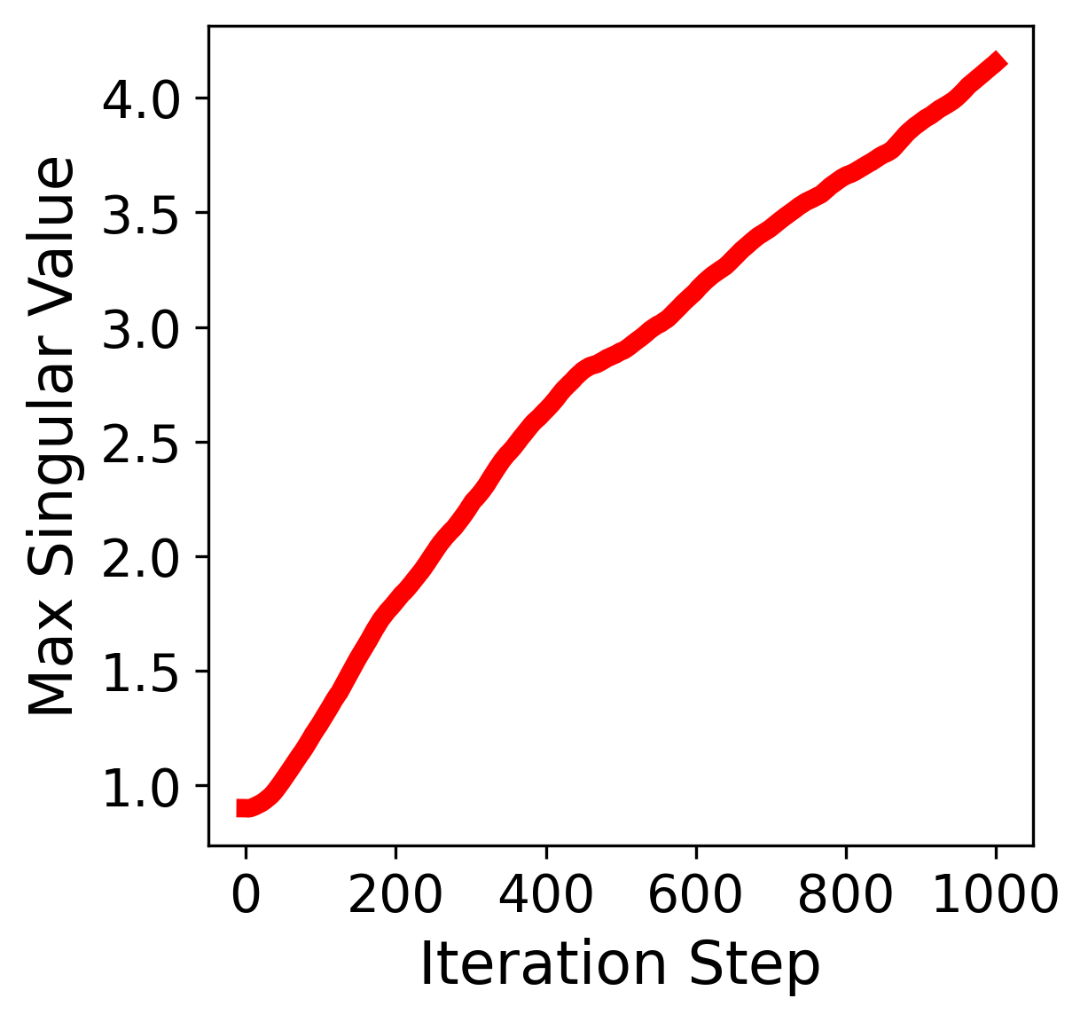
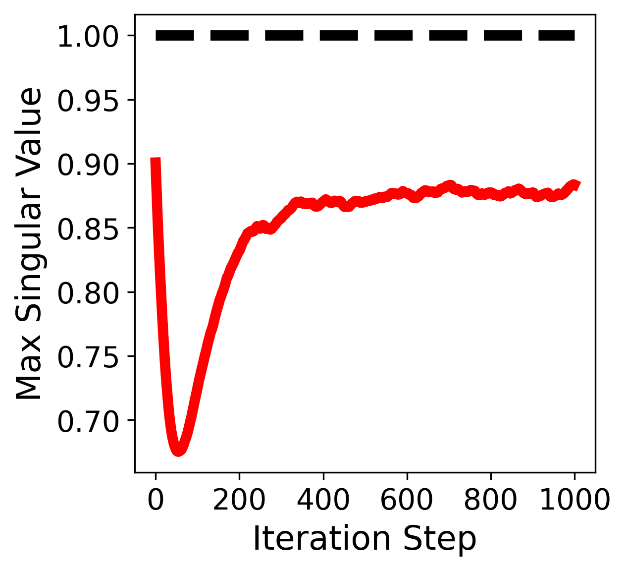
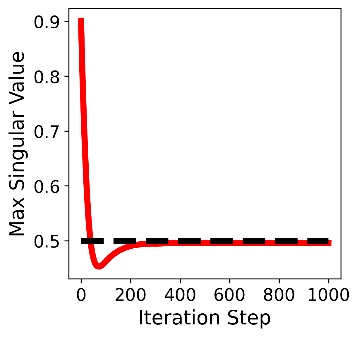
Figure: Maximum singular value \(\sigma_{\max}(X)\) vs. iteration when using Muon with different weight decay coefficients \(\lambda\).

Generalizing to Proposition 1 for Lion, the constraint enforcement property holds for any update of form \(X_{t+1} = X_t + \epsilon(O_t - \lambda X_t)\), where the update \(O_t\) is bounded in any notion of norm.

Proposition 2

Consider any update of form \(X_{t+1} = X_t + \epsilon(O_t - \lambda X_t)\) with \(\mnorm{O_t}\leq b\) and \(\epsilon \lambda \leq 1\), where \(\mnorm{\cdot}\) is any notion of norm (such as \(\mnorm{\cdot}_\infty\)), and \(b\) is a constant. Then for we have

\[ %\Phi(X_t) \mnorm{X_{t}} - \frac{b}{\lambda} \leq (1 - \epsilon \lambda)^t \left (\mnorm{X_{0}} - \frac{b}{\lambda } \right). %\Phi(X_0). \]

Hence, if the constraint \(\mnorm{X_{0}} \leq \frac{b}{\lambda}\) is satisfied, it will remain so after the update, although \(\mnorm{X_{0}}\) may increase toward the bound \(\frac{b}{\lambda}\). On the other hand, if the constraint is not initially satisfied (i.e., \(\mnorm{X_{0}} > \frac{b}{\lambda}\)), the magnitude of the violation, given by \(\mnorm{X_{0}} - \frac{b}{\lambda}\), will decrease at least geometrically.

Proof. The proof follows the same idea as the one for Proposition 1.

\[\begin{split}\begin{aligned} \mnorm{X_{t+1}} - b/\lambda & = \mnorm{(1-\epsilon\lambda ) X_{t} + \epsilon O_t} - b/\lambda \\ & \leq (1-\epsilon \lambda ) \mnorm{X_{t}} + \epsilon \mnorm{O_t} - b/\lambda \\ %~~~~~~~~ {\textcolor{magenta}{\text{//triangle inequality}}} \\ %\text{{magenta}`This sentence is blue.`} & \leq (1-\epsilon \lambda ) \mnorm{X_{t}} + \epsilon b - b/\lambda \\ %~~~~~~~~ { \textcolor{magenta}{\text{//$\mnorm{O_t} \leq b$}} }\\ & = (1-\epsilon \lambda)(\mnorm{X_{t}} -b/\lambda). \end{aligned}\end{split}\]

Applying this recursively yields the result.

Matrix Spectral Functions

We can take \(\mathcal{K}\) to be a general matrix spectral function. Let \(g\colon [0,\infty)\to\mathbb{R}\) be a scalar function. Then one may define

\[ \mathcal{K}({X}) = \sum_i g\bigl(\sigma_i(X)\bigr). \]

Because \(\frac{\partial \sigma_i(X)}{\partial X} = u_i v_i ^\top\), where \(u_i, v_i\) are the singular vectors associated with \(\sigma_i\), the derivative of \(\nabla\mathcal{K}(X)\) above is given by

\[ \nabla\mathcal{K}({X}) = {U}\,\operatorname{diag}\Bigl(\{\nabla g(\sigma_i)\}\Bigr)\,{V}. \]

where \({X}={U}\,{\Sigma}\,{V}\) is the SVD decomposition with \({\Sigma}=\operatorname{diag}\bigl(\{\sigma_i\}_i \bigr).\)

Assume \(g\) is upper bounded by \(b\), i.e., \(\sup_{x\geq 0}g(x) = b\), then the update \(O_t = \nabla \mathcal{K}(\tilde{{M}}_{t+1})\) satisfies \(\mnorm{O_t}_\infty \leq b\). This yields a constraint of \(\mnorm{X}_\infty \leq b/\lambda\) following Proposition 2.

In the practical implementation of Muon, \(g\) is effectively taken as a high order polynomial motivated with Newton-Schulz iteration for calculating the matrix sign.

Norm Constraints

More generally, the constrained optimization problem \(\min_X \mathcal{F}(X) \ \text{s.t.} \ X \in \mathcal{D}\), where \(\mathcal{D}\) is a convex set, can be solved using Lion-\(\mathcal{K}\) with \(\mathcal{K}^*(X) = \delta(X \in \mathcal{D})\). As in the cases of Lion and Muon, a particularly important instance is when \(\mathcal{D}\) is a norm ball, i.e., \(\mathcal{D} = \{X : \mnorm{X} \leq 1\}\) for some chosen norm \(\mnorm{\cdot}\). In this setting, \(\nabla \mathcal{K}(X)\) corresponds to the solution of a linear minimization oracle problem \(\max_Z \left\{ \langle X, Z \rangle \ \text{s.t.} \ \mnorm{Z} \leq 1 \right\}\). Related discussions can be found, for example, in [BN24] and [PXA+25].

Related Algorithms

To illustrate the roles of different components of Lion-\(\mathcal{K}\), we demonstrate how Lion-\(\mathcal{K}\) can be progressively constructed step by step, starting from vanilla gradient descent.

Gradient Descent

Let us start with vanilla gradient descent:

\[ X_{t+1} = X_t - \epsilon \nabla \mathcal{F}(X_t), \]

where the update direction corresponds to the steepest local descent in a neighborhood measured by the standard Euclidean distance:

\[ - \eta \nabla \mathcal{F}(X_t) = \arg\min_{V} \langle \nabla \mathcal{F}(X_t), V \rangle + \frac{1}{2\epsilon} \|V\|_2^2. \]

Dual Space Preconditioning

Adding \(\nabla \mathcal{K}(\cdot)\) to gradient descent yields a dual space preconditioning [MPTD21] algorithm:

\[ x_{t+1} = x_t + \epsilon \nabla \mathcal{K}(-\nabla \mathcal{F}(x_t)). \]

This can be viewed as a generalization of the steepest descent interpretation of gradient descent, since the update direction can be induced by

\[ \epsilon \nabla \mathcal{K}(-\nabla \mathcal{F}(x_t)) = \arg\min_{V} \left \{ \langle \nabla \mathcal{F}(X_t), V \rangle + \epsilon \mathcal{K}^*( \frac{1}{\epsilon} V) \right \} , \]

where the convex conjugate function \(\mathcal{K}^*\) is used to measure the magnitude of the update \(V\). To see the proof, note that the zero gradient equation yields \(\nabla \mathcal{F}(X_t) + \nabla \mathcal{K}^*( \frac{1}{\epsilon} V) = 0\), and using that \(\nabla\mathcal{K}^*\) is the inverse function of \(\nabla\mathcal{K}\) yields the result.

Frank-Wolfe

Adding weight decay to dual space preconditioning yields

\[ X_{t+1} = X_t + \epsilon\left( \nabla \mathcal{K}(-\nabla f(X_t)) - \lambda X_t \right). \]

This can be recognized as a Frank-Wolfe method (a.k.a. conditional gradient descent) applied to the regularized problem:

\[ \min_{X} \left\{ \mathcal{F}(X) + \frac{1}{\lambda} \mathcal{K}^*(\lambda X) \right\}. \]

Thus, the effect of weight decay, when combined with the \(\nabla \mathcal{K}\) mapping, is to introduce the convex conjugate \(\mathcal{K}^*\) as a regularization term.

The connection to the Frank-Wolfe algorithm becomes evident by rewriting the update as

\[\begin{split} \begin{aligned} Z_{t+1} &= \arg\min_{X'} \left \{ \langle \nabla \mathcal{F}(X_t), X' - X_t \rangle + \frac{1}{\lambda} \mathcal{K}^*(\lambda X') \right\}, \\ X_{t+1} &= X_t + \epsilon \lambda (Z_{t+1} - X_t), \end{aligned} \end{split}\]

where the update direction \(Z_{t+1}\) is obtained by linearizing the objective \(\mathcal{F}(X)\) while keeping the regularization/constraint term \(\frac{1}{\lambda} \mathcal{K}^*(\lambda X)\) unchanged. The final update is then taken as a convex combination of \(Z_{t+1}\) and \(X_t\), in which the weight decay term shows up.

Polyak and Nesterov Momentum

Returning to gradient descent, we replace the gradient \(\nabla \mathcal{F}(X_t)\) with Polyak momentum. It yields

\[\begin{split} \begin{aligned} & M_{t+1} = \beta_{\texttt{polyak}} M_t - (1-\beta_{\texttt{polyak}}) \nabla \mathcal{F}(X_t), \\ & X_{t+1} = X_t + \epsilon M_{t+1}. \end{aligned} \end{split}\]

This uses an exponential moving average instead of the current gradient as the update direction.

Further, Nesterov momentum is obtained by using a linear combination of the Polyak momentum and the gradient to update the parameters:

\[\begin{split} \begin{aligned} & M_{t+1} = \beta_{\texttt{polyak}} M_t - (1-\beta_{\texttt{polyak}}) \nabla \mathcal{F}(X_t), \\ & X_{t+1} = X_t + \epsilon (\beta_{\texttt{nesterov}} M_{t+1} - (1-\beta_{\texttt{nesterov}}) \nabla \mathcal{F}(X_t)). \end{aligned} \end{split}\]

Unlike the steepest descent approaches, with the introduction of momentum, the update directions no longer decreases the objective function \(\mathcal F(X)\) monotonically, as momentum introduces an inertia-like effect. To analyze the convergence with momentum, it is necessary to introduce an auxiliary Lyapunov function. To simplify the analysis, we consider the continuous-time limit of the updates. In particular, in the limit of an infinitesimal step size \(\epsilon \to 0\), the Nesterov update can be modeled by the following ODE:

\[\begin{split} \begin{aligned} & \frac{d}{dt} M_t = - \nabla \mathcal{F}(X_t) - M_t, \\ & \frac{d}{dt} X_t = M_t - \varepsilon \nabla \mathcal{F}(X_t). \end{aligned} \end{split}\]

This update does not necessarily guarantee a monotonic decrease in the original loss function \(\mathcal{F}(X)\). However, it does decrease the following auxiliary function:

\[ \mathcal{H}(X, M) = \mathcal{F}(X) + \frac{1}{2} \|M\|_2^2. \]

This can be viewed as a total energy (a.k.a. Hamiltonian function) in physics, where \(\mathcal{F}\) is the “potential energy” and \(\frac{1}{2} \|M\|_2^2\) is a “kinetic energy”. To see that \(\mathcal{H}(X, M)\) is non-increasing along the ODE, we only need to compute its time derivative:

\[\begin{split} \begin{aligned} \frac{d}{dt} \mathcal{H}(X_t, M_t) &= \langle \nabla \mathcal{F}(X_t), \frac{d}{dt} X_t \rangle + \langle M_t , \frac{d}{dt} M_t \rangle \\ &= \langle \nabla \mathcal{F}(X_t), M_t - \varepsilon \nabla \mathcal{F}(X_t) \rangle + \langle M_t, - \nabla \mathcal{F}(X_t) - M_t \rangle \\ &= - \|M_t\|_2^2 - \varepsilon \|\nabla \mathcal{F}(X_t)\|_2^2 \leq 0. \end{aligned} \end{split}\]

This shows that \(\mathcal{H}(X_t, M_t)\) yields a Lyapunov function of the dynamics, which can be used to verify the asymptotic convergence of both Polyak and Nesterov momentum algorithm. The contribution of the Nesterov momentum is reflected in the \(\varepsilon \|\nabla \mathcal{F}(X_t)\|_2^2\) term.

Hamiltonian Descent

Applying the monotonic map \(\nabla \K(\cdot)\) on Polayk momentum yields

(2)\[\begin{split}\begin{aligned} & \frac{d}{dt} M_t = - \nabla \mathcal{F}(X_t) - M_t, \\ & \frac{d}{dt} X_t = \nabla \K( M_t ). \end{aligned}\end{split}\]

This is known as Hamiltonian descent [MPT+18]. It yields a Lyapunov function of form:

\[ \mathcal{H}(X, M) = \mathcal{F}(X) + \mathcal K(M). \]

where the kinetic energy is replaced by \(\mathcal K(M)\). It is monotonically decreasing along the ODE (2):

\[\begin{split} \begin{aligned} \frac{d}{dt} \mathcal{H}(X_t, M_t) &= \langle \nabla \mathcal{F}(X_t), \frac{d}{dt} X_t \rangle + \langle \nabla \K(M_t) , \frac{d}{dt} M_t \rangle \\ &= \langle \nabla \mathcal{F}(X_t), \nabla \K(M_t) \rangle + \langle\nabla \K( M_t), - \nabla \mathcal{F}(X_t) - M_t \rangle \\ &= - \langle \nabla K(M_t), M_t \rangle \leq 0, \end{aligned} \end{split}\]

where the last inequality holds if \(\nabla \mathcal K(0) = 0\), by the monotonicity of \(\nabla \mathcal K\) that \( \langle \nabla \K(X) - \nabla \K(Y), X - Y\rangle \geq 0\) with \(X=M_t\) and \(Y = 0\).

Further, applying \(\nabla \K(\cdot)\) on Nesterov momentum yields

\[\begin{split} \begin{aligned} & \frac{d}{dt} M_t = - \nabla \mathcal{F}(X_t) - M_t, \\ & \tilde{M}_t = M_t - \varepsilon \nabla \mathcal{F}(X_t) \\ & \frac{d}{dt} X_t = \nabla \K( \tilde M_t). \end{aligned} \end{split}\]

It yields the same Lyapunov function as Hamiltonian descent:

\[\begin{split} \begin{aligned} \frac{d}{dt} \mathcal{H}(X_t, M_t) &= \langle \nabla \mathcal{F}(X_t), \frac{d}{dt} X_t \rangle + \langle M_t , \frac{d}{dt} M_t \rangle \\ &= \langle \nabla \mathcal{F}(X_t), \nabla \K(M_t - \varepsilon \nabla \mathcal{F}(X_t)) \rangle + \langle \nabla \K(M_t), - \nabla \mathcal{F}(X_t) - M_t \rangle \\ &= - \frac{1}{\varepsilon} \langle \tilde{M}_t - M_t, \nabla \K(\tilde{M}_t ) - \nabla \K (M_t) \rangle - \langle \nabla \K(M_t), M_t\rangle \leq 0, \end{aligned} \end{split}\]

where the last inequality used \(\langle \tilde{M}_t - M_t, \nabla \K(\tilde{M}_t ) - \nabla \K (M_t) \rangle \geq 0\) and \( \langle \nabla \K(M_t), M_t\rangle \geq 0\), both derived from the monotonic property of \(\nabla \K\).

Lion-\(\mathcal{K}\)

Finally, the Lion-\(\mathcal{K}\) update is obtained by putting everything together:

\[\begin{split} \begin{aligned} \text{Lion-}\mathcal{K}\text{ (ODE):}\quad \dot{{M}}_t &= -\nabla\mathcal{F}({X}_t) - {M}_t,\\[1mm] \dot{{X}}_t &= \nabla\mathcal{K}\Bigl({M}_t - \varepsilon\bigl(\nabla\mathcal{F}({X}_t) + {M}_t\bigr)\Bigr) - \lambda\,{X}_t. \end{aligned} \end{split}\]

Its Lyapunov function is somewhat more complicate:

\[ \begin{aligned} \mathcal{H}({X}, {M}) = \hat{\mathcal{F}}({X}) + \frac{1 - \varepsilon}{1 + \varepsilon \lambda} \mathcal{D}({M}, \lambda {X}), ~~~~~~~~ \text{where}~~~~~~~~~~ \mathcal{D}({M}, \lambda {X}) = {\mathcal{K}}^*(\lambda {X}) + {\mathcal{K}}({M}) - \langle {M}, \lambda {X} \rangle. \end{aligned} \]

The key complication is that the kinetic energy \(\mathcal{D}({M}, \lambda {X}) \) now depends on \({X}\) and \({M}\). This is called to be non-separable in Hamiltonian dynamics literature.

The monotonicity can be verified as follows:

(3)\[\begin{split}\begin{aligned} \frac{d}{dt} \mathcal{H}(X_t, M_t) &= \langle \nabla \mathcal{F}(X_t), \frac{d}{dt} X_t \rangle + \langle M_t , \frac{d}{dt} M_t \rangle \\ & = -\frac{1 + \lambda }{1 + \varepsilon\lambda} \Delta_1(X_t, \tilde{M}_t) - \frac{1 - \varepsilon}{1 + \varepsilon\lambda} \Delta_2(M_t, \tilde{M}_t) \leq 0, \end{aligned}\end{split}\]

where we define \(\tilde{M}_t = M_t - \varepsilon ( \nabla \mathcal{F}(X_t) + M_t)\), and

\[ \Delta_1(X_t, \tilde{M}_t) = \langle \tilde{M}_t - \nabla \K^*(\lambda X_t), \nabla \K(\tilde{M}_t) - \lambda X_t \rangle \geq 0, \]

\[ \Delta_2(M_t, \tilde{M}_t) = \frac{1}{\varepsilon} \langle \tilde{M}_t - M_t, \nabla \K(\tilde{M}_t) - \nabla \K(M_t) \rangle \geq 0. \]

The inequality \(\Delta_2(X_t, \tilde{M}_t) \geq 0\) is a direct result of monotonicity of \(\nabla \K\). The inequality \(\Delta_1(X_t, \tilde{M}_t) \geq 0\) is less obvious, but also results from the monotonicity of \(\nabla \K\) combined with \(\nabla \K(\nabla \K^*(X)) = X\):

\[ \langle X - \nabla \K^*(Y), \nabla \K(X) - Y\rangle = \langle X - \nabla \K^*(Y), \nabla \K(X) - \nabla \K(\nabla \K^*(Y)) \rangle \geq 0, \]

where the monotonicity is applied on \(X\) and \(\nabla \K^*(Y).\)

For step by step derivation of (3), see the paper [CLLL23] for the details.

Algorithm	\(\mathcal K\)	Momentum	Nesterov	Weight Decay
Polyak Momentum	\(\mathcal{K}(\mathbf{X}) = \frac{1}{2} \|\mathbf{X}\|_2^2\)	Yes	No	No
Nesterov Momentum	\(\mathcal{K}(\mathbf{X}) = \frac{1}{2} \|\mathbf{X}\|_2^2\)	Yes	Yes	No
Signed Gradient	\(\mathcal{K}(\mathbf{X}) = \|\mathbf{X}\|_1\)	No	No	No
Signed Momentum	\(\mathcal{K}(\mathbf{X}) = \|\mathbf{X}\|_1\)	Yes	Yes	No
Lion	\(\mathcal{K}(\mathbf{X}) = \norm{\mathbf{X}}_1\)	Yes	Yes	Yes
Muon	\(\mathcal{K}(\mathbf{X}) = \mnorm{\mathbf{X}}_1\)	Yes	Yes	Yes
Dual Space Preconditioning	General	No	No	No
Frank-Wolfe	General	No	No	Yes
Hamiltonian Descent	General	Yes	No	No

References

[JJB+24] (1,2)

Keller Jordan, Yuchen Jin, Vlado Boza, Jiacheng You, Franz Cesista, Laker Newhouse, and Jeremy Bernstein. Muon: an optimizer for hidden layers in neural networks. 2024. URL: https://kellerjordan.github.io/posts/muon/.

[LSY+25] (1,2)

Jingyuan Liu, Jianlin Su, Xingcheng Yao, Zhejun Jiang, Guokun Lai, Yulun Du, Yidao Qin, Weixin Xu, Enzhe Lu, Junjie Yan, and others. Muon is scalable for llm training. arXiv preprint arXiv:2502.16982, 2025.

[CLLL23] (1,2,3,4)

Lizhang Chen, Bo Liu, Kaizhao Liang, and Qiang Liu. Lion secretly solves constrained optimization: as lyapunov predicts. arXiv preprint arXiv:2310.05898, 2023.

[CLH+23] (1,2)

Xiangning Chen, Chen Liang, Da Huang, Esteban Real, Kaiyuan Wang, Hieu Pham, Xuanyi Dong, Thang Luong, Cho-Jui Hsieh, Yifeng Lu, and Quoc V Le. Symbolic discovery of optimization algorithms. Advances in neural information processing systems, 36:49205–49233, 2023.

[BN24]

Jeremy Bernstein and Laker Newhouse. Old optimizer, new norm: an anthology. arXiv preprint arXiv:2409.20325, 2024.

[PXA+25]

Thomas Pethick, Wanyun Xie, Kimon Antonakopoulos, Zhenyu Zhu, Antonio Silveti-Falls, and Volkan Cevher. Training deep learning models with norm-constrained lmos. arXiv preprint arXiv:2502.07529, 2025.

[MPTD21]

Chris J Maddison, Daniel Paulin, Yee Whye Teh, and Arnaud Doucet. Dual space preconditioning for gradient descent. SIAM Journal on Optimization, 31(1):991–1016, 2021.

[MPT+18]

Chris J Maddison, Daniel Paulin, Yee Whye Teh, Brendan O'Donoghue, and Arnaud Doucet. Hamiltonian descent methods. arXiv preprint arXiv:1809.05042, 2018.