		Search-engine friendly clone of the ACL2 documentation.

Vwsim-tutorial

Vwsim-tutorial-2

VWSIM tutorial: Simulating a Josephson Transmission Line.

In this tutorial, we demonstrate how to use VWSIM to simulate a Rapid Single Flux Quantum (RSFQ) circuit. We will model, simulate, and analyze a "Josephson Transmission Line" (JTL). A JTL accepts a RSFQ fluxon (bit) as input and transmits the fluxon from the input to the output. Let's simulate our first RSFQ circuit!

Preparing VWSIM

Prior to analyzing models with VWSIM, see vwsim-build-and-setup for build instructions. To simulate a circuit, start ACL2 and then load the simulator:

(ld "driver.lsp")

Read and Simulate the Circuit Description

We will simulate a simple JTL circuit with the SPICE description shown below. This circuit is composed of three subcircuit definitions and a top-level circuit. The first subcircuit, damp_jj, describes a Josephson junction (JJ) in parallel with a "damping" resistor (or external shunt). The second subcircuit, bias, describes a bias current source, which is defined to be a voltage source in series with a resistor. The final subcircuit, jtl4, is the definition of our JTL, which uses the subcircuits we defined. jtl4 is a four-stage JTL since the fluxon passes through four JJs before reaching the output. The top-level circuit provides fluxons every 20 picoseconds to the JTL, which then provides the output to a resistor.

Schematic of the four-stage JTL subcircuit

Schematic of the top-level circuit

SPICE description

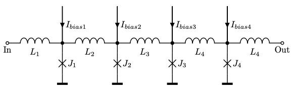
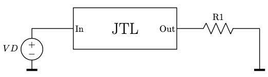
* A hand-written, SPICE description of a four-stage JTL.

*** The model line provides some of the Josephson junction (JJ)
*** parameters.
.model jmitll jj(rtype=1, vg=2.8mV, cap=0.07pF, r0=160, rN=16, icrit=0.1mA)

*** Overdamped JJ subcircuit

.subckt damp_jj pos neg
BJi pos neg jmitll area=2.5
RRi pos neg 3
.ENDS damp_jj

*** Bias current source subcircuit

.SUBCKT bias out gnd
RR1 NN out 17
VrampSppl@0 NN gnd pwl (0 0 1p 0.0026V)
.ENDS bias

*** Four-stage JTL subcircuit

.SUBCKT jtl4 in out gnd
LL1 in net@1 2pH
XJ1 net@1 gnd damp_jj
Xbias1 net@1 gnd bias

LL2 net@1 net@2 2pH

XJ2 net@2 gnd damp_jj
Xbias2 net@2 gnd bias
LL3 net@2 net@3 2pH

XJ3 net@3 gnd damp_jj
Xbias3 net@3 gnd bias
LL4 net@3 net@4 2pH

XJ4 net@4 gnd damp_jj
Xbias4 net@4 gnd bias
LL5 net@4 out 2pH

.ENDS jtl4

*** TOP LEVEL CIRCUIT

* Pulses at 5p, 25p, ...
VD D gnd pulse (0 0.6893mV 5p  1p 1p 2p 20p)
Xjtl4d D out gnd jtl4

RR1 out gnd 5

.END

A copy of this description can be found in "Testing/test-circuits/cirs/four-stage-jtl.cir".

Note that the SPICE description file does not contain a .tran command! That is, it does not provide a simulation start time, simulation step size, and stop time. In fact, VWSIM does not require this information to be provided in the SPICE file. The start time, stop time, simulation step size, and several other options can be provided directly as input arguments to the simulator.

We will simulate the JTL circuit from 0 seconds to 100 picoseconds with a step size of 1/10 of a picosecond.

VWSIM can simulate the JTL circuit using the following command:

(vwsim "Testing/test-circuits/cirs/four-stage-jtl.cir"
            :time-step (* 1/10 *pico*)
            :time-stop (* 100 *pico*))

The arguments to the command above are as follows. The first argument to VWSIM is the file that contains the SPICE description of the JTL circuit. The second argument is the time step size, :time-step. For the time step size, we provide a LISP expression that will evaluate to a number. In this case, (* 1/10 *pico*) evaluates to 1/10 of a picosecond. Check out vwsim-constants for a list of in-built constants that VWSIM provides. Note that instead of (* 1/10 *pico*), we could have provided the number 1/10000000000000. The final argument is the time to stop the simulation, :time-stop, which is 100 picoseconds. The command above will then read the specified VWSIM circuit model, and attempt to parse, flatten, initialize, and simulate the JTL model. If there is any processing error, VWSIM will stop the process at that point.

Inspect Simulation Results

As the JTL circuit model is simulated, VWSIM stores the simulation values for each time step. Upon completion, we can request specific simulation results. In this case, we would like to inspect whether our JTL is working as intended. We can look at the phase across each JJ in the JTL and determine whether they fired (i.e. the phase across the JJ steps up or down by 2*pi). Using the vw-output-command, we can inspect the phase across each JJ in the JTL. We will store these phases in the global variable jj-phases.

(vw-output '((PHASE . BJi/XJ1/XJTL4D)
             (PHASE . BJi/XJ2/XJTL4D)
             (PHASE . BJi/XJ3/XJTL4D)
             (PHASE . BJi/XJ4/XJTL4D))
              :save-var 'jj-phases)

The output result is an alistp. We can inspect the phase-time values across each JJ in the ACL2 loop by executing the following command:

(@ jj-phases)

Depending on the length of the simulation, this can be a lot to print out! We can instead visualize the simulation results using a graphing utility.

Save and Plot Simulation Results

Using the vw-output-command, we can write the phases across each JJ to a comma-separated values (CSV) file. A time-value graph of signal values can be plotted; e.g., using GNUplot.

(vw-output '((PHASE . BJi/XJ1/XJTL4D)
             (PHASE . BJi/XJ2/XJTL4D)
             (PHASE . BJi/XJ3/XJTL4D)
             (PHASE . BJi/XJ4/XJTL4D))
           :output-file "Testing/test-circuits/csvs/four-stage-jtl.csv")

VWSIM provides the vw-plot-command to run gnuplot from the ACL2 prompt. Here, we plot the phase across each JJ with respect to time.

(vw-plot '((PHASE . BJi/XJ1/XJTL4D)
           (PHASE . BJi/XJ2/XJTL4D)
           (PHASE . BJi/XJ3/XJTL4D)
           (PHASE . BJi/XJ4/XJTL4D))
         "Testing/test-circuits/csvs/four-stage-jtl.csv")

Analyze Simulation Results

At this point, it is up to the user to view the plotted results to determine whether the desired results were achieved. In the next tutorial example, we will demonstrate how to write an ACL2 program to analyze a simulation result.

Previous: Simulating a simple circuit

Next: Simulating an RSFQ D-latch