		Search-engine friendly clone of the ACL2 documentation.

Vwsim-tutorial

Vwsim-tutorial-3

VWSIM tutorial: Simulating an RSFQ D-latch.

In this tutorial, we will model, simulate, and analyze a Rapid Single Flux Quantum (RSFQ) "D-latch" circuit. A D-latch offers a mechanism to store a single fluxon (bit) in the RSFQ logic. The D-latch we define will have two input wires (D, C) and one output wire (Out). The D input requests the latch to store a fluxon. The C input requests the latch to release the stored fluxon through Out. If there is no fluxon stored in the latch, then a fluxon is not released through Out.

Preparing VWSIM

Prior to analyzing models with VWSIM, see vwsim-build-and-setup for build instructions. To simulate a circuit, start ACL2 and then load the simulator:

(ld "driver.lsp")

Read and Simulate the Circuit Description

We will simulate a D-latch circuit with the SPICE description shown below. This circuit is composed of 4 subcircuit definitions and a top-level circuit. The first subcircuit, damp_jj, describes a Josephson junction (JJ) in parallel with a "damping" resistor (or external shunt). The second subcircuit, bias, describes a bias current source, which is defined to be a voltage source in series with a resistor. The third subcircuit, jtl4, is a four-stage JTL transmission line. These three subcircuits are the same circuits defined in the previous tutorial vwsim-tutorial-2. The final subcircuit, D_latch, defines the D latch we will simulate. A diagram of the D latch is shown below. The top-level circuit provides fluxons through pulse generators. The generators are connected to Josephson Transmission Lines (JTLs), which then connect to either the D or C input of the D latch. The D latch Out output wire is also connected to a JTL, which provides the output fluxons to a resistor.

Schematic of the D-latch subcircuit

Schematic of the top-level circuit

SPICE description

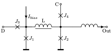
* A hand-written, SPICE description of an RSFQ D-latch.

*** The model line provides some of the Josephson junction (JJ)
*** parameters.
.model jmitll jj(rtype=1, vg=2.8mV, cap=0.07pF, r0=160, rN=16, icrit=0.1mA)

*** Overdamped JJ subcircuit

.SUBCKT damp_jj pos neg
BJi pos neg jmitll area=2.5
RRi pos neg 3
.ENDS damp_jj

*** Bias current source subcircuit

.SUBCKT bias out gnd
RR1 NN out 17
VrampSppl@0 NN gnd pwl (0 0 1p 0.0026V)
.ENDS bias

*** 4-stage JTL subcircuit

.SUBCKT jtl4 in out gnd
LL1 in net@1 2pH
XJ1 net@1 gnd damp_jj
Xbias1 net@1 gnd bias

LL2 net@1 net@2 2pH

XJ2 net@2 gnd damp_jj
Xbias2 net@2 gnd bias
LL3 net@2 net@3 2pH

XJ3 net@3 gnd damp_jj
Xbias3 net@3 gnd bias
LL4 net@3 net@4 2pH

XJ4 net@4 gnd damp_jj
Xbias4 net@4 gnd bias
LL5 net@4 out 2pH

.ENDS jtl4

*** D Latch circuit

.SUBCKT D_latch D C out gnd
XJ3 D net@1 damp_jj
XJ1 net@1 gnd damp_jj
Xbias1 net@1 gnd bias

LL net@1 net@2 12pH

XJ4 C net@2 damp_jj
XJ2 net@2 gnd damp_jj
LY net@2 out 2pH
.ENDS D_latch

*** TOP LEVEL CIRCUIT

* Fluxon pulses at 20p, 70p, ...
VD D gnd pulse (0 0.6893mV 20p 1p 1p 2p 50p)
Xjtl4d D rD gnd jtl4

* Fluxon pulses at 5p, 55p, ...
VC C gnd pulse (0 0.6893mV 5p 1p 1p 2p 50p)
Xjtl4c C rC gnd jtl4

* Create instance of D latch subcircuit
XD_latch rD rC out gnd D_latch

* Output JTL
Xjtl_latch out out2 gnd jtl4
RR1 out2 gnd 5

.END

A copy of this description can be found in "Testing/test-circuits/cirs/d-latch.cir".

Note that the SPICE description file does not contain a .tran command! That is, it does not provide a simulation start time, simulation step size, and stop time. In fact, VWSIM does not require this information to be provided in the SPICE file. The start time, stop time, simulation step size, and several other options can be provided directly as input arguments to the simulator.

We will simulate the D-latch circuit from 0 seconds to 100 picoseconds with a step size of 1/10 of a picosecond.

VWSIM can simulate the JTL circuit using the following command:

(vwsim "Testing/test-circuits/cirs/d-latch.cir"
            :time-step (* 1/10 *pico*)
            :time-stop (* 100 *pico*))

The arguments to the command above are as follows. The first argument to VWSIM is the file that contains the SPICE description of the D-latch circuit. The second argument is the time step size, :time-step. For the time step size, we provide a LISP expression that will evaluate to a number. In this case, (* 1/10 *pico*) evaluates to 1/10 of a picosecond. Check out vwsim-constants for a list of in-built constants that VWSIM provides. Note that instead of (* 1/10 *pico*), we could have provided the number 1/10000000000000. The final argument is the time to stop the simulation, :time-stop, which is 100 picoseconds. The command above will then read the specified VWSIM circuit model, and attempt to parse, flatten, initialize, and simulate the JTL model. If there is any processing error, VWSIM will stop the process at that point.

Inspect Simulation Results

As the D-latch circuit model is simulated, VWSIM stores the simulation values for each time step. Upon completion, we can request specific simulation results. We would like to inspect whether our D-latch is working as intended. We can look at the current through the quantizing inductor (LL) in the D-latch. When there is a fluxon (bit) in the D-latch, there will be a larger current circulating in the J1-LL-J2 loop than when there is no fluxon stored in the latch. Using the vw-output-command, we can inspect the current through inductor LL in the D-latch. We will store these currents in the global variable ll-currents.

(vw-output '((DEVI . LL/XD_LATCH))
           :save-var 'll-currents)

The output result is an alistp. We can inspect the current-time values through LL in the ACL2 loop by executing the following command:

(@ ll-currents)

Depending on the length of the simulation, this can be a lot to print out! We can instead visualize the simulation results using a graphing utility.

Save and Plot Simulation Results

Using the vw-output-command, we can write the current through LL to a comma-separated values (CSV) file. A time-value graph of signal values can be plotted; e.g., using GNUplot.

(vw-output '((DEVI . LL/XD_LATCH))
           :output-file "Testing/test-circuits/csvs/d-latch.csv")

VWSIM provides the vw-plot-command to run gnuplot from the ACL2 prompt. Here, we plot the phase across each JJ with respect to time.

(vw-plot '((DEVI . LL/XD_LATCH))
         "Testing/test-circuits/csvs/d-latch.csv")

Analyze Simulation Results

Since all of the simulation results are already available in the loop, we can perform analysis on the circuit. We will identify when a fluxon passes through the Josephson junction J1, which suggests that a fluxon is stored in the D-latch.

We need to inspect the phase across J1 at all simulation times and determine when a fluxon passes through the JJ. This will be when the phase across the JJ has stepped up or down by a multiple of 2*pi (i.e. when the phase across the JJ has completed a full "turn" around the unit circle). To perform this analysis, consider the following function definitions.

(defun detect-fluxon-through-jj-recur (jj-phases times turns)
  ;; check if list of phases is empty
  (if (atom jj-phases)
      nil
    (let* (;; get next phase across the JJ
           (phase (car jj-phases))
           (2pi (* 2 (f*pi*)))
           (new-turns (truncate phase 2pi)))
      (if ;; detect a step up/down in 2pi phase across the JJ
          (not (= new-turns turns))
          ;; full fluxon detected
          (cons (car times)
                (detect-fluxon-through-jj-recur
                 (cdr jj-phases) (cdr times) new-turns))
        ;; full fluxon through the jj yet
        (detect-fluxon-through-jj-recur
         (cdr jj-phases) (cdr times) turns)))))

(defun detect-fluxon-through-jj (jj-phases times)
  ;; check if list of phases is empty
  (if (atom jj-phases)
      nil
    (let* ((2pi (* 2 (f*pi*)))
           ;; calculate how many times the JJ has already been turned
           ;; by 2pi radians
           (initial-phase (car jj-phases))
           (initial-turn (truncate initial-phase 2pi)))
      ;; find all times a fluxon passed through the JJ (i.e. the JJ
      ;; turned)
      (detect-fluxon-through-jj-recur
       (cdr jj-phases) (cdr times) initial-turn))))

The detect-fluxon-through-jj function takes two input arguments: a list of the phases across the JJ for each simulation time step and a list of the simulation times for each simulation time step. Then it determines how many times the phase across the JJ has already been turned at the beginning of the simulation. Then, it calls the function detect-fluxon-through-jj-recur which recurs through the rest of the phases and records each time the phase across the JJ completes a full turn.

Before we can run these functions, we need to define these function definitions in ACL2. Copy and paste the two function definitions above into your ACL2 session.

We need to provide the phase across J1 for each time step and the list of simulation times for each time step to our detect-fluxon-through-jj function. We will access the phase values from the output alist produced by the vw-output-command using the vw-assoc-command. vw-assoc takes as input a key-value pair (in this case, we are requesting the phase across J1) and an alist produced by vw-output. It then returns the requested key along with its simulation values, if the key exists in the alist, otherwise it returns NIL. We can take the cdr of the list produced by vw-assoc to remove the key from the front of the list.

We can now execute the following two commands:

(vw-output '((PHASE . BJi/XJ1/XD_LATCH))
           :save-var 'loop-phases)

(detect-fluxon-through-jj
 (cdr (vw-assoc '(PHASE . BJi/XJ1/XD_LATCH) (@ loop-phases)))
 (cdr (vw-assoc '$time$ (@ loop-phases))))

which results in

(3.11e-11 8.11e-11)

This means that, during the simulation, a fluxon passed through J1 at 31 picoseconds and 81 picoseconds. We can check whether this is what we expected. The pulse generators produce a pulse on the D input at 20 picoseconds and 70 picoseconds, and on the C input at 5 picoseconds and 55 picoseconds. This sequence requests the latch to be emptied at 5 picoseconds, filled at 20 picoseconds, emptied at 55 picoseconds, and filled at 70 picoseconds. Our analysis is consistent with this description. A fluxon passed through J1 every time the latch was filled (20ps and 70ps). Note: the ~11 picosecond delay from request to the fluxon passing through J1 is primarily due to the time it takes for the fluxons to pass through the four-stage JTLs before reaching the latch.

This concludes the tutorial. You can navigate to the vwsim-users-guide to learn more about the different simulator options.

We hope you enjoy VWSIM. Happy simulating!

Previous: Simulating a Josephson Transmission Line