Linearly Separable?

Which Digit?

Introduction

In this project, you will implement the perceptron algorithm and gradient descent, which you will use to train neural network classifiers. You will come up with hand-designed features, and also train a convolutional neural network to learn even better features. You will test your learned classifiers on a set of scanned handwritten digit images.

Optical character recognition (OCR) is the task of extracting text from image sources. The data set on which you will run your classifiers is a collection of handwritten numerical digits (0-9). This is a very commercially useful technology, similar to the technique used by the US post office to route mail by zip codes. There are systems that can perform with over 99% classification accuracy (see LeNet-5 for an example system in action).

The code for this project includes the following files and data, available as a zip file.

Files to Edit and Submit: You will fill in portions of perceptron.py, answers.py, solvers.py, search_hyperparams.py and features.py (only) during the assignment, and submit them. You should submit these files with your code and comments along with the others in the distribution.

Evaluation: Your code will be autograded for technical correctness. Please do not change the names of any provided functions or classes within the code, or you will wreak havoc on the autograder. However, the correctness of your implementation -- not the autograder's judgements -- will be the final judge of your score. If necessary, we will review and grade assignments individually to ensure that you receive due credit for your work.

Academic Dishonesty: We will be checking your code against other submissions in the class for logical redundancy. If you copy someone else's code and submit it with minor changes, we will know. These cheat detectors are quite hard to fool, so please don't try. We trust you all to submit your own work only; please don't let us down. If you do, we will pursue the strongest consequences available to us.

Getting Help: You are not alone! If you find yourself stuck on something, contact the course staff for help. Office hours, section, and the discussion forum are there for your support; please use them. If you can't make our office hours, let us know and we will schedule more. We want these projects to be rewarding and instructional, not frustrating and demoralizing. But, we don't know when or how to help unless you ask.

Discussion: Please be careful not to post spoilers.

QUESTION 1 (4 POINTS): Perceptron

A skeleton implementation of a perceptron classifier is provided for you in perceptron.py. In this part, you will fill in the train function inside the PerceptronClassifier class.

Unlike the naive Bayes classifier, a perceptron does not use probabilities to make its decisions. Instead, it keeps a weight vector \(w^y\) of each class \(y\) ( \(y\) is an identifier, not an exponent). Given a feature list \(f\), the perceptron compute the class \(y\) whose weight vector is most similar to the input vector \(f\). Formally, given a feature vector \(f\) (in our case, a map from pixel locations to indicators of whether they are on), we score each class with:

Then we choose the class with highest score as the predicted label for that data instance. In the code, we will represent \(w^y\) as a Counter.

Learning weights

In the basic multi-class perceptron, we scan over the data, one instance at a time. When we come to an instance \((f, y)\), we find the label with highest score:

We compare \(y'\) to the true label \(y^*\). If \(y' = y^*\), we've gotten the instance correct, and we do nothing. Otherwise, we guessed \(y'\) but we should have guessed \(y^*\). That means that \(w^{y^*}\) should have scored \(f\) higher, and \(w^{y'}\) should have scored \(f\) lower, in order to prevent this error in the future. We update these two weight vectors accordingly:

Using the addition, subtraction, and multiplication functionality of the Counter class in util.py, the perceptron updates should be relatively easy to code. Certain implementation issues have been taken care of for you in perceptron.py, such as handling iterations over the training data and ordering the update trials. Furthermore, the code sets up the weights data structure for you. Each legal label needs its own Counter full of weights.

Question

Fill in the train method in perceptron.py. Run your code with:

python dataClassifier.py --model PerceptronModel 

Hints and observations:

• The command above should yield validation and test accuracies in the range between 70% to 85%. These ranges are wide because the perceptron is sensitive to the specific choice of tie-breaking.
• One of the problems with the perceptron is that its performance is sensitive to several practical details, such as how many iterations you train it for, and the order you use for the training examples (in practice, using a randomized order works better than a fixed order). The current code uses a default value of 10 training iterations. You can change the number of iterations for the perceptron with the --iter [iterations] option. Try different numbers of iterations and see how it influences the performance. In practice, you would use the performance on the validation set to figure out when to stop training, but you don't need to implement this stopping criterion for this assignment.
• You should use the most of up-to-date weights when you classify the datum as you iterate over the data (i.e. the inner for loop).

QUESTION 2 (1 POINT): Perceptron Convergence

Question

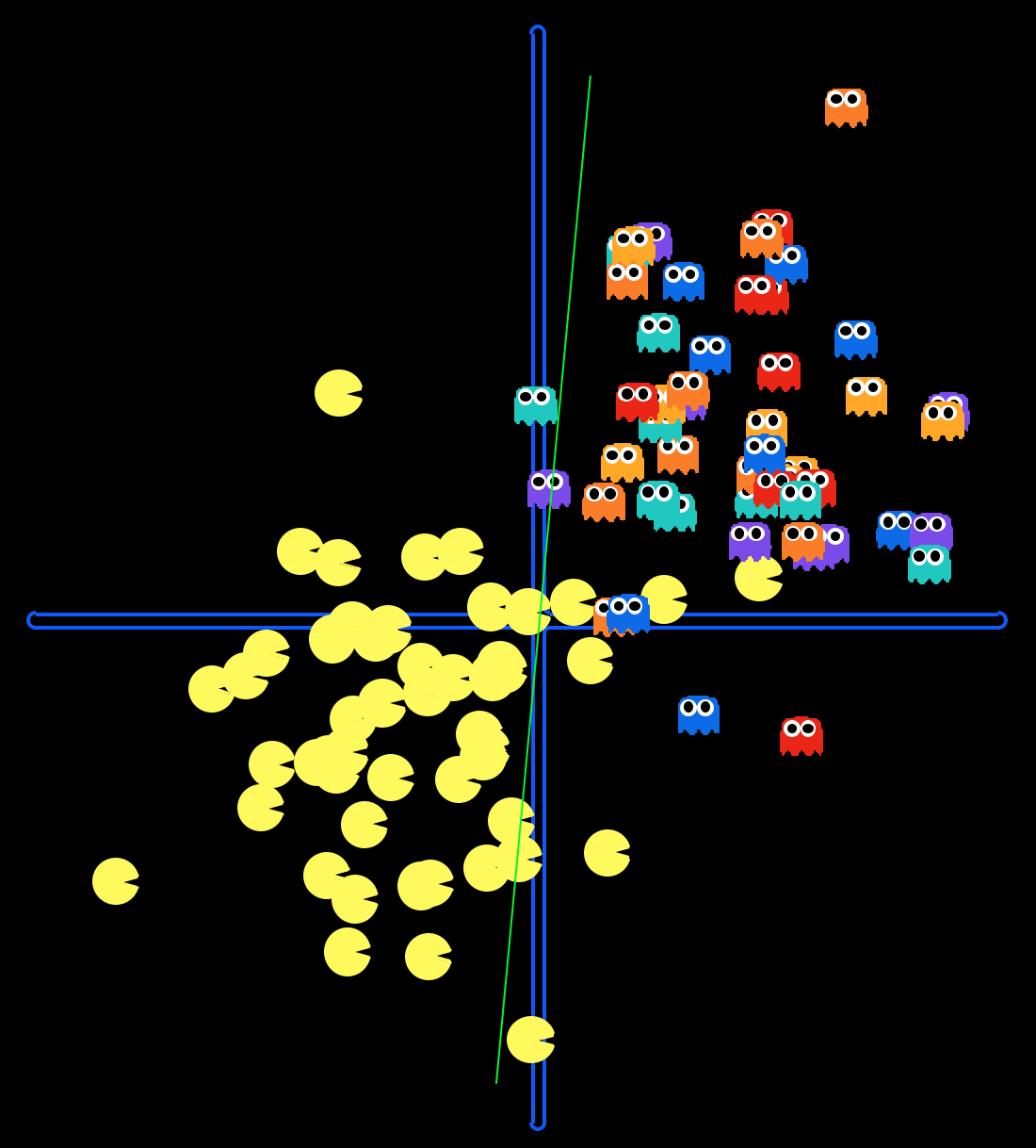
Visualize the Perceptron's training process on two 2D data sets by running the following commands:

python dataClassifier.py --model PerceptronModel --data datasetA --iter [iterations]

python dataClassifier.py --model PerceptronModel --data datasetB --iter [iterations]

You should replace [iterations] with the number of iterations the perceptron will run for.

For which datasets does the Perceptron not converge?

Answer this question by returning either 'none', 'a', 'b', or 'both' in the q2 method of answers.py.

QUESTION 3 (1 POINT): Perceptron Analysis

Visualizing weights

Perceptron classifiers, and other discriminative methods, are often criticized because the parameters they learn are hard to interpret. To see a demonstration of this issue, we can write a function to find features that are characteristic of one class.

Question

Fill in find_high_weight_features(self, label) in perceptron.py. It should return a list of the 100 features with highest weight for that label. If you implement find_high_weight_features(self, label) correctly, you can display the 100 pixels with the largest weights using the command:

python dataClassifier.py --model PerceptronModel --print_features --iter 1  

Use this command to look at the weights, and answer the following question. Which of the following sequence of weights is most representative of the perceptron?

(a)
(b)

Answer this question by returning either 'a' or 'b' in method q3 in answers.py.

TUTORIAL (0 POINTS): TensorFlow

For the next questions, you will be using TensorFlow to train neural net models and testing them. We have put together a short tutorial to go over the basic concepts of TensorFlow. You can find the code used in this tutorial in the script tutorial.py. Feel free to take a look at the TensorFlow tutorial if you want to learn more about it.

If you don't have TensorFlow installed already, you can run pip install tensorflow --user on a CS lab machine or simply pip install tensorflow on your own machine.

If you prefer to install within a virtual environmnet on a CS lab machine, then:

1. mkdir tensorflow
2. virtualenv --system-site-packages tensorflow
3. source ~/tensorflow/bin/activate
4. easy_install -U pip
5. pip install --upgrade tensorflow
6. To run tensorflow, run source ~/tensorflow/bin/activate. You can deactivate the virtualenv with the command: deactivate

If both these options fail, follow TensorFlow's installation instructions. If your installation was successful, you should be able to import tensorflow without getting any errors. We will also be using the numpy library.

>>> import tensorflow as tf
>>> import numpy as np

Ops and Tensors

TensorFlow is a programming system in which you represent computations as graphs. Nodes in the graph are called ops (short for operations). An op takes Tensors, performs some computation, and produces Tensors. A Tensor is a typed multi-dimensional array whose value may depend on other Tensors. For example, you can represent a mini-batch of images as a 4D array of floating point numbers with dimensions [batch, height, width, channels].

Computation Graph and Session

A TensorFlow graph is a description of computations. To compute anything, a graph must be launched in a Session. A session places the graph ops onto Devices, such as CPUs or GPUs, and provides methods to execute them. TensorFlow programs are usually structured into a construction phase that assembles a graph, and an execution phase that uses a session to execute ops in the graph. For example, it is common to create a graph to represent the training of a neural network in the construction phase, and then repeatedly execute a set of training ops in the graph in the execution phase.

Placeholders

We start building the computation graph by creating nodes for the input images.

>>> x_ph = tf.placeholder(tf.float32, shape=(2, 1))

Here x_ph does not have an specific value. It is a placeholder—an object that will be replaced by a tensor when we run a computation involving that placeholder. Even though a placeholder does not have an specific tensor value, its type must be specified and its dimensions (also known as shape) can optionally be specified. It's typical in deep learning to use 32-bit floating point numbers since the additional precision of 64-bit numbers is unnecessary. In addition, some of the dimensions of the shape can remain unknown by specifying None instead of a size. For instance, a shape of (2, None) indicates that this placeholder could take the value of a 2-dimensional tensor where its first dimension has to be 2 and its second dimension could be any size.

Variables

We now define the weight matrices W_var and biases b_var, which are the parameters of our model. We could imagine treating these like additional inputs, but TensorFlow has an even better way to handle them: Variable. A Variable is a value that lives in TensorFlow's computation graph. It can be used and even modified by the computation. In machine learning applications, one generally has the model parameters be Variables. We pass the initial value for each parameter when instantiating each variable. These values are numpy.arrays, which are the standard way of representing tensors values.

>>> W_var = tf.Variable(np.array([[1, 0], [0, 1], [1, 0], [0, 1]]), dtype=tf.float32)
>>> b_var = tf.Variable(np.array([[1], [1], [-1], [-1]]), dtype=tf.float32)

Tensor

Unlike numpy.arrays, which represent actual tensor values, TensorFlow's Tensor may depend on placeholders and variables instead of having a particular value. That is, it could be evaluated to a numpy.array when the session is run.

>>> y_tensor = tf.matmul(W_var, x_ph) + b_var

Variable Initialization

We initialize both W_var and b_var as tensors from some numpy.array. Before variables can be used within a session, they must be initialized using that session. This step takes the initial values that have already been specified, and assigns them to each variable. This can be done for all variables at once.

>>> session = tf.Session()
>>> session.run(tf.initialize_all_variables())

You don't need to initialize any variables in your project since all the variables are already initialized for you.

Session

You can evaluate placeholders, variables, tensors and ops by passing them to session.run. For example, we can evaluate W_var.

>>> W_value = session.run(W_var)
>>> print('W_value:\n%r' % W_value)
W_value:
array([[ 1.,  0.],
       [ 0.,  1.],
       [ 1.,  0.],
       [ 0.,  1.]], dtype=float32)

However, if you try to evaluate y_tensor without passing any other arguments, an error is raised since you need to specify a numpy.array to be used to replace the placeholder x_ph.

>>> y_value = session.run(y_tensor)
...
tensorflow.python.framework.errors.InvalidArgumentError: You must feed a value for placeholder tensor 'Placeholder' with dtype float and shape [2,1]
...

To do it correctly, you should pass in a dictionary mapping placeholders to the numpy.arrays they should replace. You should use the keyword argument feed_dict to specify such dictionary.

>>> x_datum = np.array([[3], [7]])
>>> y_value = session.run(y_tensor, feed_dict={x_ph: x_datum})
>>> print('x_datum:\n%r\ny_value:\n%r' % (x_datum, y_value))
x_datum:
array([[3],
       [7]])
y_value:
array([[ 4.],
       [ 8.],
       [ 2.],
       [ 6.]], dtype=float32)

More on session

You can also specify ops to be performed when running the session. For instance, W2_op is an op that updates W_var to be twice its value.

>>> W2_op = tf.assign(W_var, W_var*2)

You can pass a list to session.run to do multiple evaluations at a time. So, if you pass in [y_tensor, W2_op], y_tensor is evaluated again and W_var is updated to be twice as much. The return values of session.run are the evaluated numpy.arrays of the corresponding elements in the list that was passed in.

>>> y_value, W2_value = session.run([y_tensor, W2_op], feed_dict={x_ph: x_datum})
>>> print('y_value:\n%r\nW2_value:\n%r' % (y_value, W2_value))
y_value:
array([[ 4.],
       [ 8.],
       [ 2.],
       [ 6.]], dtype=float32)
W2_value:
array([[ 2.,  0.],
       [ 0.,  2.],
       [ 2.,  0.],
       [ 0.,  2.]], dtype=float32)

When y_tensor is evaluated again, it is using the new value of W_var.

>>> y2_value = session.run(y_tensor, feed_dict={x_ph: x_datum})
>>> print('y2_value:\n%r' % y2_value)
y2_value:
array([[  7.],
       [ 15.],
       [  5.],
       [ 13.]], dtype=float32)

QUESTION 4 (2 POINTS): Gradient Descent Updates

In this question and the following ones, you will be implementing a gradient descent optimizer, and variants of it, to train neural networks. Neural networks are implemented as Models and the optimizers are implemented as Solvers.

Models

A neural net is represented by a Model, which contains a TensorFlow's computation graph to compute the output of the network. This output depends on the inputs and on the parameters \(w\) of the network, which are represented as TensorFlow's placeholders and variables, respectively. A few models (linear regression, softmax regression and convolutional neural net models) have already been provided for you in models.py, so you shouldn't need to modify anything in that file. The parameters of these model will be optimized using a Solver. You will be implementing a few solvers in solvers.py.

Solvers

The Solver addresses the general optimization problem of loss minimization. The typical loss (also known as objective) is the average loss over all \(m\) data points throughout the dataset,

\( ll(w) = \frac{1}{m} \sum\limits_{i=1}^{m} ll_i(w) + \lambda r(w) \),

where \(ll_i(w)\) is the loss on data point \(x^{(i)} \) and \(r(w)\) is a regularization term with weight \(\lambda\) (also known as weight decay). Typical losses include the squared error loss for regression, \( ll_i(w) = ||y^{(i)} - f(x^{(i)}; w)||^2 \), and the categorical crossentropy for classification, \( ll_i(w) = -\sum_c y^{(i)}_c \log(f_c(x^{(i)}; w)) \), where \(f\) is the neural net function and \(c\) are the categories. The regularization term on the weights (e.g. the \(\ell 2\) norm \(r(w) = ||w||_2^2\)) is typically included in the loss to help prevent overfitting to the training data.

The size of the dataset, \(m\), can be very large, so in practice, we use a stochastic approximation of the objective in each solver iteration by drawing a mini-batch of \(k << m\) instances,

\( ll(w) \approx \frac{1}{k} \sum\limits_{i=1}^{k} ll_i(w) + \lambda r(w) \).

The loss \( ll(w) \) can be optimized using the gradient descent optimization algorithm. When the stochastic approximation of the loss is used, the algorithm is called stochastic gradient descent.

Gradient Descent Updates

Gradient descent (and its stochastic variations) updates the model parameters \(w\) by substracting it by the gradient of the loss, \(\nabla ll(w)\), weighted by the learning rate \(\alpha\).

Formally, we have the following formula to compute the updated parameters \(w_{t+1}\) at iteration \(t+1\), given the current parameters \(w_t\):

\( w_{t+1} = w_t - \alpha \nabla ll(w_{t}) \)

The learning hyperparameter \(\alpha \) has to be chosen and it might require a bit of tuning.

Question

Fill in the get_updates_without_momentum method in solvers.py, which implements the parameter updates above. This method should return a list of tuples, each tuple being the parameter variable to be updated and the updated parameter tensor, (\(w_t, w_{t+1})\). To run the autograder for this question:

python autograder.py -q q4

Hints and observations:

• You should use the member variable self.learning_rate for the learning rate \(\alpha\).
• Applying an operation to a TensorFlow Variable results in a TensorFlow Tensor.

QUESTION 5 (1 POINT): Gradient Descent Updates with Momentum

In this question, you will add momentum to the gradient descent update. In this setting, the model parameters \(w\) are updated with a linear combination of the negative gradient \(\nabla ll(w_t)\) and the previous weight update \(v_t\). The learning rate \(\alpha\) is the weight of the negative gradient and the momentum \(\mu\) is the weight of the previous update.

Formally, we have the following formulas to compute the updated value \(v_{t+1}\) and the updated weights \(w_{t+1}\) at iteration \(t+1\), given the previous weight update \(v_t\) and current weights \(w_t\):

\( v_{t+1} = \mu v_t - \alpha \nabla ll(w_t) \)

\( w_{t+1} = w_t + v_{t+1} \)

The learning hyperparameters \(\alpha\) and \(\mu\) have to be chosen and it might require a bit of tuning. Notice that in the extreme case when \(\mu = 0\), the update becomes the update that you implemented in question 4.

Question

Fill in the get_updates_with_momentum method in solvers.py, which implements the updates above. As before, this method should return a list of tuples, each tuple being the variable to be updated and the updated variable tensor. To run the autograder for this question:

python autograder.py -q q5

Hints and observations:

• You should use the member variables self.learning_rate and self.momentum for the learning rate \(\alpha\) and the momentum \(\mu\), respectively.
• Applying an operation to a TensorFlow Variable results in a TensorFlow Tensor.
• The TensorFlow's variables vel_vars correspond to the variables \(v_t\) of each parameter of the model.
• The returned updates should include updates of the the variables \(v_t\).

QUESTION 6 (4 POINTS): Gradient Descent

In this question you will implement gradient descent and its stochastic variants.

Question 6a (2 points): Gradient Descent

Fill in the solve method of the GradientDescentSolver class in solvers.py, which implements the gradient descent algorithm. That is, in every iteration of the algorithm, the parameters should be updated using the gradient of the loss of all the training data. Read the method's docstring for specific details of what you should do for this part. To run the autograder for this part:

python autograder.py -q q6a

Question 6b (1 point): Stochastic Gradient Descent

Fill in the solve method of the StochasticGradientDescentSolver class in solvers.py, which implements the stochastic gradient descent algorithm. That is, in every iteration of the algorithm, the parameters should be updated using the gradient of the loss of only one data point of the training data. Read the method's docstring for specific details of what you should do for this part. To run the autograder for this part:

python autograder.py -q q6b

Question 6c (1 point): Minibatch Stochastic Gradient Descent

Fill in the solve method of the MinibatchStochasticGradientDescentSolver class in solvers.py, which implements the gradient descent algorithm. That is, in every iteration of the algorithm, the parameters should be updated using the gradient of the loss of a batch of the training data. Read the method's docstring for specific details of what you should do for this part. To run the autograder for this part:

python autograder.py -q q6c

Hints and observations:

• Unlike the perceptron algorithm where a single iteration corresponds to iterating over the whole dataset once, a single iteration in StochasticGradientDescentSolver and MinibatchStochasticGradientDescentSolver corresponds to a single update of the parameters.
• You must use the MinibatchIndefinitelyGenerator class provided for you to iterate over the data. This class shuffles the data for you and indefinitely iterates over the data (possibly iterating through the dataset multiple times).
• For every iteration, the training loss should be evaluated with the weights before updating them, but the validation loss should be evaluated with the weights after updating them.
• You should call run.session(...) exactly two times per iteration.

QUESTION 7 (1 POINT): Softmax Regression Convergence

Instead of using the perceptron algorithm, we are now minimizing a loss function with optimization techniques. Does this approach improve convergence?

Question

Visualize the Softmax Regression's training process on two 2D data sets by running the following commands:

python dataClassifier.py --model SoftmaxRegressionModel --data datasetA --iter [iterations]

python dataClassifier.py --model SoftmaxRegressionModel --data datasetB --iter [iterations]

You should replace [iterations] with the number of iterations Softmax Regression will run for.

For which datasets does Softmax Regression converge?

Answer the question this question in the q7 method of answers.py returning either 'none', 'a', 'b', or 'both'.

QUESTION 9 (5 POINTS): Digit Feature Design

Building classifiers is only a small part of getting a good system working for a task. Indeed, the main difference between a good classification system and a bad one is usually not the classifier itself (e.g. perceptron vs. softmax regression), but rather the quality of the features used. So far, we have used the simplest possible features: the identity of each pixel (being on/off). You can see the classifier run with this set of features by running the following command:

python dataClassifier.py --data largeMnistDataset --feature_extractor basicFeatureExtractor --iter 1000 --learning_rate 0.01 --momentum 0.9

To increase your classifier's accuracy further, you will need to extract more useful features from the data. The enhancedFeatureExtractor in features.py is your new playground. When analyzing your classifiers' results, you should look at some of your errors and look for characteristics of the input that would give the classifier useful information about the label. You can add code to the analysis function in features.py to inspect what your classifier is doing. For instance in the digit data, consider the number of separate, connected regions of white pixels, which varies by digit type. 1, 2, 3, 5, 7 tend to have one contiguous region of white space while the loops in 6, 8, 9 create more. The number of white regions in a 4 depends on the writer. This is an example of a feature that is not directly available to the classifier from the per-pixel information. If your feature extractor adds new features that encode these properties, the classifier will be able exploit them. Note that some features may require non-trivial computation to extract, so write efficient and correct code.

Question

Add new features for the digit dataset in the enhancedFeatureExtractor function. Note that you can encode a feature which takes 3 values [1, 2, 3] by using 3 binary features, of which only one is on at the time, to indicate which of the three possibilities you have. You can prototype your features and check the accuracy that you get with the following command:

python dataClassifier.py --data largeMnistDataset --feature_extractor enhancedFeatureExtractor --iter 1000 --learning_rate 0.01 --momentum 0.9

Running the softmax regression classifier with the basic features should yield 86.1% on the validation set and 87.0% on the test set. You must achieve an accuracy of at least 88% on the test set (of largeMnistDataset) in order to pass this question. For your reference, our implementation yields 88.0% on the validation set and 89.1% on the test set when using the features descibed above. However, you may use any features as long as you achieve an accuracy of at least 88% on the test set.

Hints and observations:

• You may want to use your new features in addition to the basic features by concatenating them all.
• The reference implementation uses the basic features (i.e. pixels being on/off) and the 3 enhanced features mentioned above (i.e. one-hot encoding representing the number of white connected components).
• Our reference implementation takes 28s in a Ubuntu 14.04 desktop (using a Titan X GPU), 900s in one of the hive machines (using a GeForce GT 740 GPU), and 82s in a MacBook Pro (using the CPU only).