Subsection 2.1.1 Low rank approximation
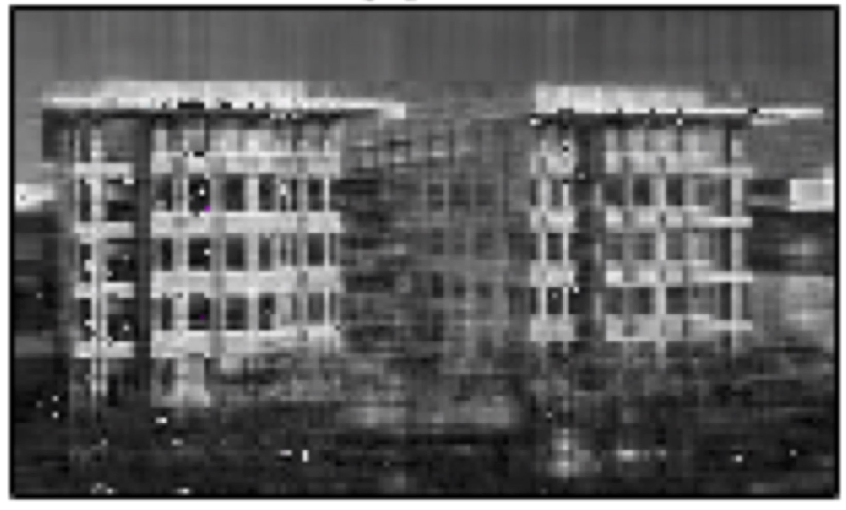
¶Consider this picture of the Gates Dell Complex that houses our Department of Computer Science:

where we recognize that we can view the picture as a matrix. What if we want to store this picture with fewer than \(m \times n \) data? In other words, what if we want to compress the picture? To do so, we might identify a few of the columns in the picture to be the "chosen ones" that are representative of the other columns in the following sense: All columns in the picture are approximately linear combinations of these chosen columns.
Let's let linear algebra do the heavy lifting: what if we choose \(k \) roughly equally spaced columns in the picture:
where for illustration purposes we assume that \(n \) is an integer multiple of \(k \text{.}\) (We could instead choose them randomly or via some other method. This detail is not important as we try to gain initial insight.) We could then approximate each column of the picture, \(b_j \text{,}\) as a linear combination of \(a_0, \ldots, a_{k-1} \text{:}\)
We can write this more concisely by viewing these chosen columns as the columns of matrix \(A \) so that
If \(A \) has linearly independent columns, the best such approximation (in the linear least squares sense) is obtained by choosing
where you may recognize \(( A^T A )^{-1} A^T \) as the (left) pseudo-inverse of \(A \text{,}\) leaving us with
This approximates \(b_j \) with the orthogonal projection of \(b_j \) onto the column space of \(A \text{.}\) Doing this for every column \(b_j \) leaves us with the following approximation to the picture:
which is equivalent to
Importantly, instead of requiring \(m \times n\) data to store \(B \text{,}\) we now need only store \(A \) and \(X \text{.}\)
Homework 2.1.1.1.
If \(B \) is \(m \times n \) and \(A \) is \(m \times k \text{,}\) how many entries are there in \(A \) and \(X \) ?
\(A \) is \(m \times k \text{.}\)
\(X \) is \(k \times n \text{.}\)
A total of \((m+n) k \) entries are in \(A \) and \(X \text{.}\)
Homework 2.1.1.2.
\(A X \) is called a rank-k approximation of \(B \text{.}\) Why?
The matrix \(A X \) has rank at most equal to \(k \) (it is a rank-k matrix) since each of its columns can be written as a linear combinations of the columns of \(A \) and hence it has at most \(k \) linearly independent columns.
Let's have a look at how effective this approach is for our picture:
original:

\(k = 1 \)

\(k = 2 \)

\(k = 10 \)

\(k = 25 \)
\(k = 50 \)

Now, there is no reason to believe that picking equally spaced columns (or restricting ourselves to columns in \(B \)) will yield the best rank-k approximation for the picture. It yields a pretty good result here in part because there is quite a bit of repetition in the picture, from column to column. So, the question can be asked: How do we find the best rank-k approximation for a picture or, more generally, a matrix? This would allow us to get the most from the data that needs to be stored. It is the Singular Value Decomposition (SVD), possibly the most important result in linear algebra, that provides the answer.
Remark 2.1.1.1.
Those who need a refresher on this material may want to review Week 11 of Linear Algebra: Foundations to Frontiers [26]. We will discuss solving linear least squares problems further in Week 4.