Subsection 7.4.2 Parallelism in splitting methods
¶One of the advantages of, for example, the Jacobi iteration over the Gauss-Seidel iteration is that the values at all mesh points can be updated simultaneously. This comes at the expense of slower convergence to the solution.
There is actually quite a bit of parallelism to be exploited in the Gauss-Seidel iteration as well. Consider our example of a mesh on a square domain as illustrated by
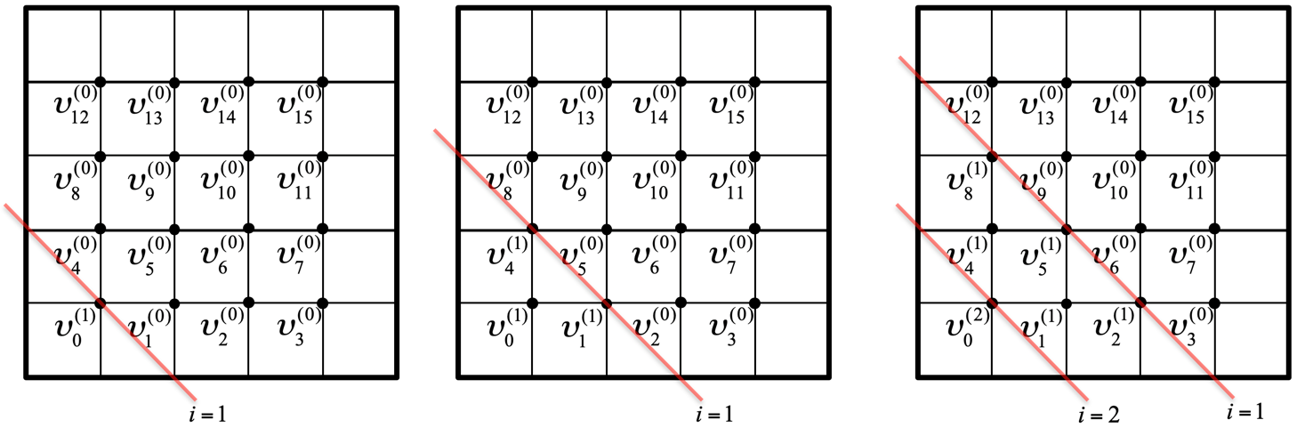
First \(\upsilon_0^{(1)} \) is computed from \(\upsilon_1^{(0)} \) and \(\upsilon_{N}^{(0)} \text{.}\)
-
Second, simultaneously,
\(\upsilon_1^{(1)} \) can be computed from \(\upsilon_0^{(1)} \text{,}\) \(\upsilon_2^{(0)} \text{,}\) and \(\upsilon_{N+1}^{(0)} \text{.}\)
\(\upsilon_N^{(1)} \) can be computed from \(\upsilon_0^{(1)} \text{,}\) \(\upsilon_{N+1}^{(0)} \text{,}\) and \(\upsilon_{2N}^{(0)} \text{.}\)
-
Third, simultaneously,
\(\upsilon_2^{(1)} \) can be computed from \(\upsilon_1^{(1)} \text{,}\) \(\upsilon_2^{(0)} \text{,}\) and \(\upsilon_{N+2}^{(0)} \text{.}\)
\(\upsilon_{N+1}^{(1)} \) can be computed from \(\upsilon_1^{(1)} \text{,}\) \(\upsilon_{N}^{0i)} \text{,}\) and \(\upsilon_{N+2}^{(0)} \text{,}\) and \(\upsilon_{2N+1}^{(0)} \text{.}\)
\(\upsilon_{2N}^{(1)} \) can be computed from \(\upsilon_{N}^{(1)} \text{,}\) and \(\upsilon_{2N+1}^{(0)} \text{,}\) and \(\upsilon_{3N}^{(0)} \text{.}\)
AND \(\upsilon_0^{(2)} \) can be computed from \(\upsilon_1^{(1)} \) and \(\upsilon_{N}^{(1)} \text{,}\) which starts a new "wave."
What we notice is that taking the opportunity to update when data is ready creates wavefronts through the mesh, where each wavefront corresponds to computation related to a different iteration.
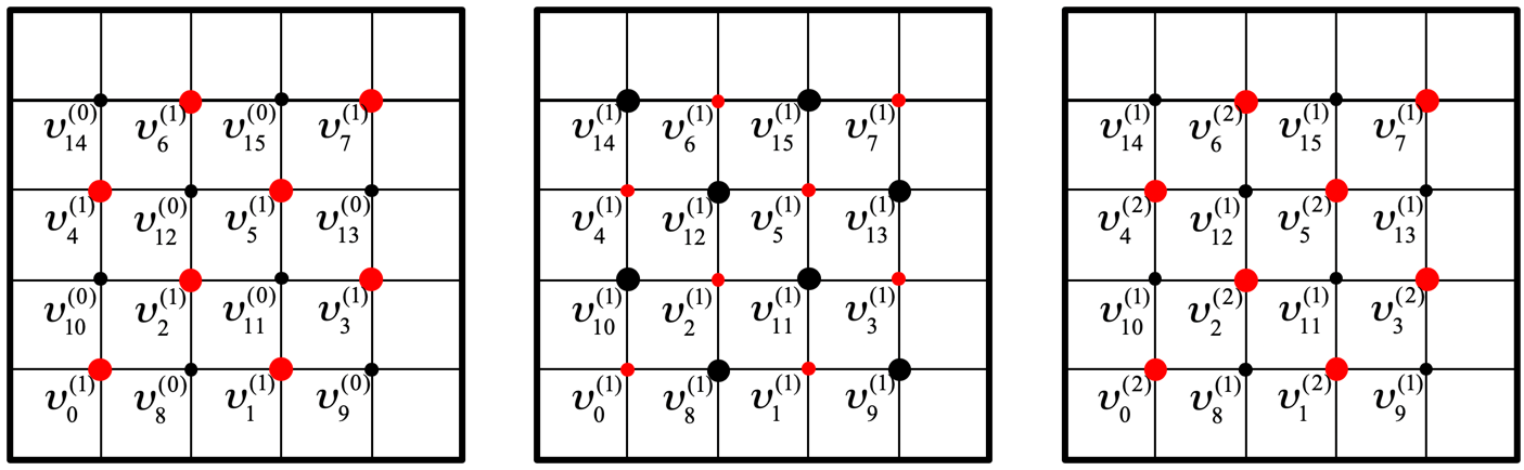
Alternatively, extra parallelism can be achieved by ordering the mesh points using what is called a red-black ordering. Again focusing on our example of a mesh placed on a domain, the idea is to partition the mesh points into two groups, where each group consists of points that are not adjacent in the mesh: the red points and the black points.