Unit 1.3.6 Matrix-matrix multiplication via matrix-vector multiplications
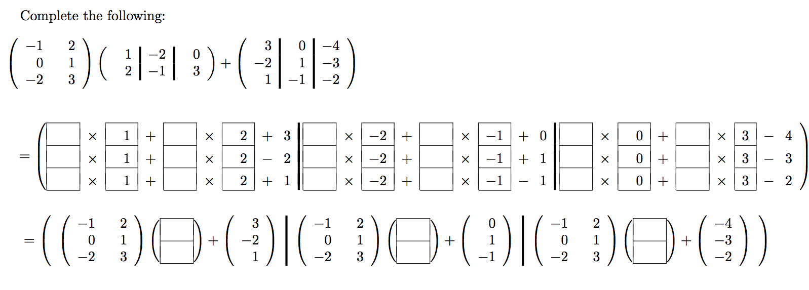
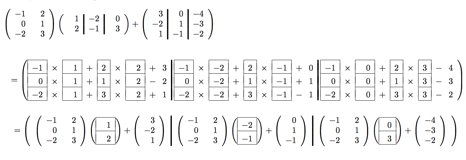
¶Homework 1.3.6.1.
Fill in the blanks:
Now that we are getting comfortable with partitioning matrices and vectors, we can view the six algorithms for \(C := A B + C \) in a more layered fashion. If we partition \(C \) and \(B \) by columns, we find that
A picture that captures this is given by
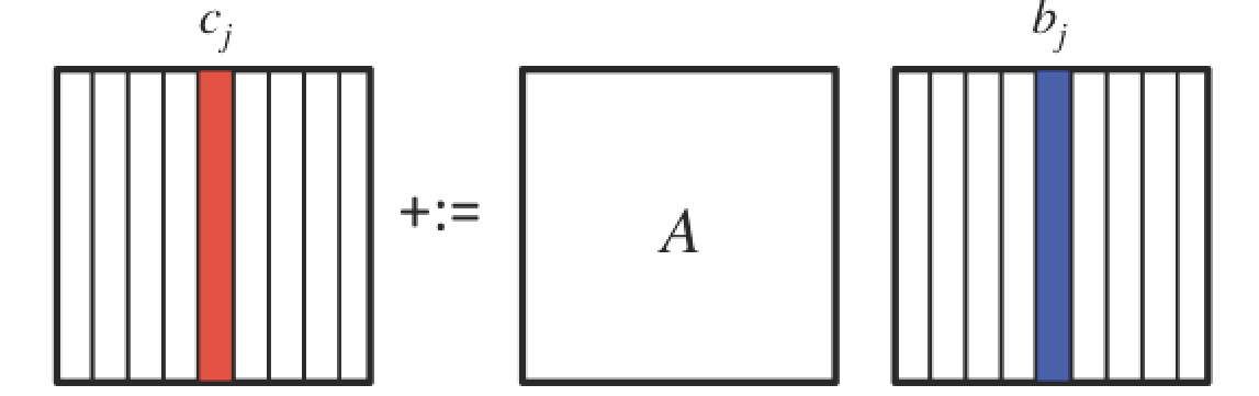
This illustrates how the JIP and JPI algorithms can be layered as a loop around matrix-vector multiplications, which itself can be layered as a loop around dot products or axpy operations:
and
Homework 1.3.6.2.
Complete the code in Assignments/Week1/C/Gemm_J_Gemv.c. Test two versions:
make J_Gemv_I_Dots
make J_Gemv_J_Axpy
View the resulting performance by making the necessary changes to the Live Script in Assignments/Week1/C/Plot_Outer_J.mlx. (Alternatively, use the script in Assignments/Week1/C/data/Plot_Outer_J_m.m.)
Remark 1.3.6.
The file name Gemm_J_Gemv.c can be decoded as follows:
The Gemm stands for "GEneral Matrix-Matrix multiplication."
The J indicates a loop indexed by \(j\) (a loop over columns of matrix \(C\)).
The Gemv indicates that the operation performed in the body of the loop is matrix-vector multiplication.
Similarly, J_Gemv_I_Dots means that the implementation of matrix-matrix multiplication being compiled and executed consists of a loop indexed by \(j\) (a loop over the columns of matrix \(C\)) which itself calls a matrix-vector multiplication that is implemented as a loop indexed by \(i\) (over the rows of the matrix with which the matrix-vector multiplication is performed), with a dot product in the body of the loop.
Remark 1.3.7.
Hopefully you are catching on to our naming convention. It is a bit adhoc and we are probably not completely consistent. They give some hint as to what the implementation looks like.
Going forward, we refrain from further explaining the convention.