Unit 2.3.4 Combining loops
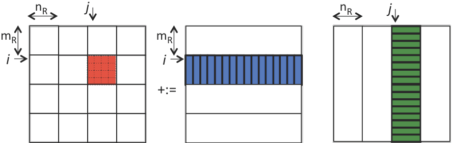
¶What we now recognize is that matrices \(A \) and \(B\) need not be partitioned into \(m_R \times k_R \) and \(k_R \times n_R \) submatrices (respectively). Instead, \(A\) can be partitioned into \(m_R \times k\) row panels and \(B\) into \(k \times n_R \) column panels:
Homework 2.3.4.1.
In directory Assignments/Week2/C copy the file Assignments/Week2/C/Gemm_JIP_P_Ger.c into Gemm_JI_P_Ger.c and remove the \(p \) loop from
MyGemm. Execute it with
make JI_P_Gerand view its performance with
Assignments/Week2/C/data/Plot_register_blocking.mlx
This is the performance on Robert's laptop, with MB=NB=KB=4:
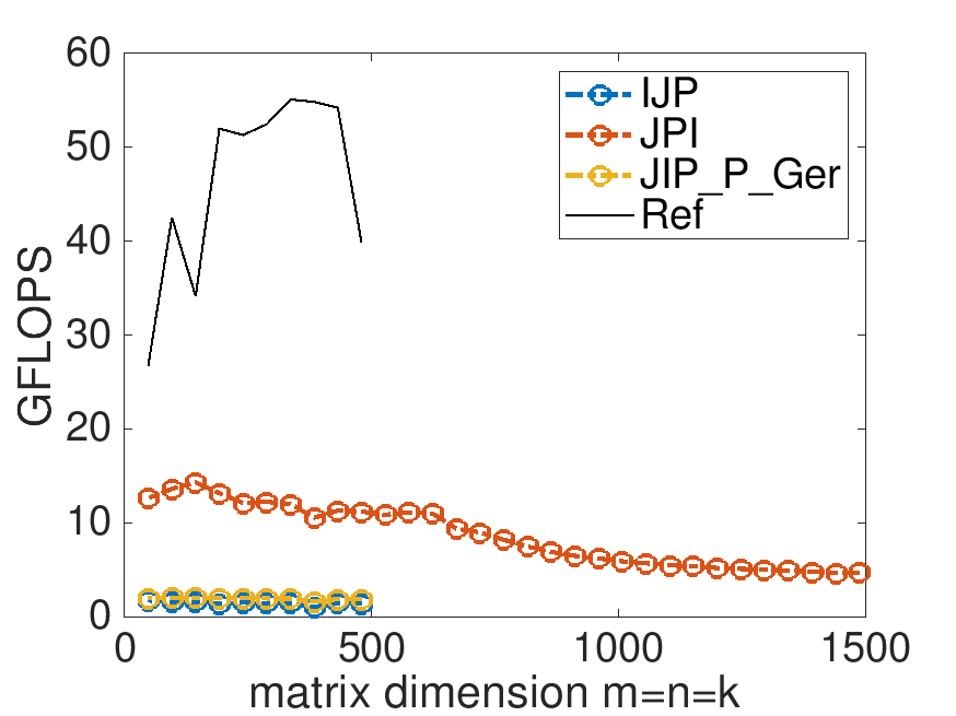
Again, it is tempting to start playing with the parameters MB, NB, and KB. However, the point of this exercise is to illustrate the discussion about how the loops indexed with \(p \) can be combined, casting the multiplication with the blocks in terms of a loop around rank-1 updates.
Homework 2.3.4.2.
In detail explain the estimated cost of the implementation in Homework 2.3.4.1.
Bringing \(A_{i,p} \) one column at a time into registers and \(B_{p,j} \) one row at a time into registers does not change the cost of reading that data. So, the cost of the resulting approach is still estimated as
Here
\(2 m n k \gamma_R \) is time spent in useful computation.
\(\left[ 2 m n + m n k ( \frac{1}{n_R} + \frac{1}{m_R} ) \right] \beta_{R \leftrightarrow M} \) is time spent moving data around, which is overhead.
The important insight is that now only the \(m_R \times n_R \) micro-tile of \(C \text{,}\) one small column \(A \) of size \(m_R \) one small row of \(B\) of size \(n_R \) need to be stored in registers. In other words, \(m_R \times n_R + m_R + n_R \) doubles are stored in registers at any one time.
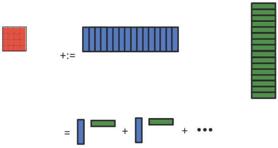
One can go one step further: Each individual rank-1 update can be implemented as a sequence of axpy operations:
Here we note that if the block of \(C \) is updated one column at a time, the corresponding element of \(B \text{,}\) \(\beta_{p,j} \) in our discussion, is not reused and hence only one register is needed for the elements of \(B \text{.}\) Thus, when \(m_R = n_R = 4 \text{,}\) we have gone from storing \(48 \) doubles in registers to \(24 \) and finally to only \(21 \) doubles.. More generally, we have gone from \(m_R n_R + m_R k_R + k_R n_R \) to \(m_R n_R + m_R + n_R \) to
doubles.
Obviously, one could have gone further yet, and only store one element \(\alpha_{i,p} \) at a time. However, in that case one would have to reload such elements multiple times, which would adversely affect overhead.