Autonomous Intersection Management: Notebook
9/8/2010
Single Intersection Observation: Serious clogs after ~1000 seconds, mainly in right and left lanes. Why don’t the cars load-balance between lanes?
2x2 Intersection Observation: Serious single-lane congestion after 150 seconds in right lanes in about half of the roads. 200 seconds show left lanes getting clogged as well. 260 seconds: one segment of road clogged on all 3 lanes. After ~300s congestion seems reasonably stable: All segments of road exiting the system are clear. Of the interior roads, all that have right turns reaching and “exit segment” are clear. All others are fully clogged.
3x3 Intersection Observation: ~300 secs the lanes entering the grid are exhibiting varying levels of congestion. The roads interior to the grid are semi-congested.
9/11/2010
Goal is to create traffic jam via sup-optimal route planning. I’ve succeeded in doing such using a 3x3 grid where all traffic spawns from the same origin and goes to the same destination. The problem is that when cars make a right turn, they all right turn into a single lane. This combines 3 lanes of traffic into a single one, creating far more traffic than would realistically occur. We need some sort of load balancing before this example can become even remotely accurate.
Changing the MAX_LANES_TO_TRY_PER_ROAD variable to 3 (rather than 1) seems to do a great job of load balancing the roads, although traffic still accumulates after some number of seconds. This is odd because even on the straightaway segments, cars will always stop and hesitate before entering the intersection and even though there is no dangerous cross-traffic they will not just go straight through as expected, which means more work is required to get a decent baseline. At a normal rate of flow of cars, there are no blockages.
I just had a revolutionary realization: to keep the autonomous intersection flowing optimally it is required that cars don’t have to stop to get into it. If all cars can simply sail through then it works optimally. Once cars have to stop and wait it gets alot worse since to start the cars again requires them to take a lot more of the intersection’s space-time. Perhaps intersections should ensure that they only take enough cars so as to not accumulate traffic.
Todo: 1. Figure out how to count cars who made it through the system 2. Random A* 3. Understand how to setup repeatable experiments
9/14/2010
Aim is to modify the A* so that it returns random equidistant solutions. This was accomplished by modifying the A* search so that the actual distance traveled estimate was simply the number of roads traversed and the estimated distance to goal was the Euclidean distance between the car’s current segment of road and the destination point. Lists of exit roads from each intersection were shuffled so as to randomize road choice (between equally good roads).
Next, lets get the average delay script running. This seems to be the main evaluation metric so it’s going to be critical. This looks to be a somewhat larger task...
9/17/2010
Initial baselining experiment: Measured average delay through a 3x3 grid of intersections for different traffic loads. All traffic spawned from the top left and traversed to the bottom right following the same route. With a traffic level of 0.3, the average delay was 3.4993seconds; a traffic load of 0.7 gave 104.8449 seconds of delay. All runs were recorded for 1000 seconds.
After modifiying the A* search so that it selects random roads to the destination, the same experiments were carried out: With a traffic load of 0.3, average delay was 2.2315 and with a traffic load of 0.7, the average delay was 70.0911 seconds.
These results seem to indicate that, as expected, the delays are reduced when each car chooses a random path through the grid rather than having all the cars use the same path.
9/18/2010
Finished creating the baseline scenario in which traffic will need to be dynamically re-directed. Essentially there is a persistent flow of traffic which is periodically interrupted by heavy flows which saturate several of the roads. The persistent flow of traffic will need to adapt to these dynamic influxes and re-route traffic along different paths.
9/25/2010
Implemented a new vehicle to intersection (v2i) message which notifies the intersection when a vehicle has arrived on a road leading to that intersection. This is useful for allowing the intersections to keep track of the number of active cars on all incoming roads. After each intersection knows the approximate incoming traffic road, this information can be used for path planning by the individual drivers. Specifically, depending on the driver's preferences (fear of traffic), she can decide to choose a shorter path to the goal or a less used one. This has proved an effective method of load balancing in the small scenarios in which incoming traffic clogs a few intersections and a persistent traffic flow must divert in order to avoid delays.
Currently struggling with some problems with A*.
9/26/2010
Fixed A* problem so it no longer returns sub-optimal routes (there was an issue with the way the remaining distance to the destination was estimated).
9/30/2010
Lecture in my Operating System course today was about overload control and made me realize that intersection management is essentially a resource allocation problem. There is a limited supply of intersection space-time. It may be possible to apply standard scheduling algorithms to the problem such as First in First Out, Round Robin, etc. The typical metric we are trying to optimize is latency (average delay). The provably optimal scheduling algorithm in this regard is to always work on the request that takes the least space-time, which is different from the current First Come First Served algorithm we are using. However, intersection management doesnt map exactly onto task scheduling because it's not possible to do some work on a request and then put it aside and work on other requests. As soon as a car enters the intersection, we will likely want to continue working on it until it has exited from the intersection.
Additionally, if you could guarantee that a car would encounter no delays when traversing the roads between intersections, it should be theoretically possible to just allow a single car to make a sequence of reservations as soon as it leaves its driveway all the way up to the destination. The problem with this is that it's not possible to guarantee that there will be no delays along the roads between intersections. Imagine the case in which there is only a single lane road connecting intersections which is currently occupied by a car driving at half the speed that you were expecting to drive at. In this case, you'd certainly miss your next reservation. Now it might be possible for the grid of intersections to detect this and incorporate it into your original route planning.
The next step would be to allow the network of intersections to optimize routes through them. Rather than allowing each car to plan its own routes and make its own reservations, the global intersection manager should take as input the car's origin and destination and plan an optimal route through the grid for that car. Note that this optimal route may not be the same as the car would have come up with itself using a greedy approach. In other words, I believe the solution space is not convex. I'm not sure about the computational complexity of scheduling cars on optimal paths to minimize some heuristic (likely average delay), but it may very well be NP-hard.
My conclusion from all this rambling is that traffic optimization so long as it remains within a network of fully autonomous intersections should be optimally solvable (at least for a small number of cars and intersections) from some central intersection manager.
10/11/2010
Over the past week I've implmented a collision detector which simply checks that no car's polygons overlap any other car. I was hoping that this was able to shed some light on the problem of occasional collisions inside intersections. Additionally, it also revealed that there are minor collisions between cars before they enter the intersection. From Chiu's advice, I fixed the intra-intersection collisions by enforcing that traffic which is going straight through the intersection only request the exit lane corresponding to their entry lane. This was causing collisions problems because when this traffic was assigned a different exit lane, the code controlling the car does not know how to switch lanes and, as a result, would drive straight through the intersection, causing a collision. Enforcing that cars going straight through the intersection only send one request qualitatively has not adversely affected the throughput of the intersection very much.
10/15/2010
Did some experiments to examine the feasibility of using regression to determine the expected delay of a given intersection knowing only the number of active cars for that intersection. By active cars, we mean the number of cars which are on direct paths to that intersection and will traverse it. To this end, I examined five different traffic scenarios on a single intersection. For each I collected data points on the number of active cars and the average delay encountered by those vehicles. The five traffic scenarios are as follows:
- Expected (Random) Case: Cars spawn from all roads and lane with random destinations. This is the typical case for an intersection.
- Favorable Case: Traffic flows in opposite directions directly past each other. There is are not turns or interruptions. Essentially, traffic can be pushed through as fast as it comes in.
- Single Merge: One lane of traffic goes straight through to the destination. Another lane of traffic merges with it and head for the same destination.
- Double Merge: Two lanes of traffic both turn to get to the same destination.
- Triple Merge: Same as double merge except we add the "straight-through" traffic back in.

The favorable case is not graphed here because there is zero delay regardless of the amount of active traffic. The other four look like they are roughly linear. However, I feel that knowing only the number of active vehicles on an intersection is not enough to predict the delay. The correct way to solve the intersection regression problem is to keep track of the delay of each car as is traverses the intersection. Then simply take the average of a sliding window. Even so, this still is perhaps too coarse (consider the case in which there is massive traffic only on a single lane of the intersection but not on other lanes). Even better would be to keep track of the average delay for each entrance, exit pair. This way when a new car requests an estimate on the delay, it will also provide the predicted entrance and exit lanes that it plans to use and the intersection can provide with a highly accurate estimate.
10/16/2010
Upon further examination, there are many different ways to solve the intersection delay estimation problem. Many of them have shortcomings and trade-offs so I will outline a few below. First, lets define the problem: we are trying to predict how long it will take for a given car to traverse some intersection. This data is useful for cars as they plan which route to take through a network of intersections. In order to create an accurate estimate there are several pieces of data we have access to:
- Number of active cars: The number of cars which are on roads leading directly to this intersection and no other intersections in between. That is, each active car has yet to traverse the intersection and will traverse it before it traverses any other intersection. We can count the total number of active cars on the whole intersection or the number of active cars on any given entrance road, exit road pair. (That is the number of cars which are going to enter the intersection through "entrance" and exit through "exit"). Some facts that we can conclude from this data: if there are no active cars on the intersection, there will be no delay. If there are lots of active cars, it is likely there will be delays for most paths through the intersection.
- List of traversals: Essentially we just keep a list of all the cars who have successfully traversed the intersection. This list should include the entrance, exit pair specifying the path that the car followed and the total amount of time taken to traverse the intersection. This can be useful for estimating future traversal times using past traversal times.
- Active Vehicle Approach: We estimate delay based on some function of the number of active vehicles on the full intersection or on a specific path through the intersection. Currently we use this approach with a simple linear function of the total number of vehicles active on that intersection. This has the advantage of dynamically adapting to incoming traffic flows. However, if we only keep track of the number of active vehicles on the full intersection we lose much data about specific paths. For example, there could be many active vehicles clogging several paths but a different path might be completely free. In this case we would want to estimate low delay for the free path and high delay for the crowded path. This cannot be done using only the #AV (number active vehicles) on the full intersection. If we switch the #AV on each path, we solve the above problem but encounter a different one: perhaps there is very little traffic on an East-West path through the intersection but heavy traffic on the North-South path. In this case the North-South traffic can interfere with the East-West traffic so our estimation of the delay of an East-West path should be nonzero. This hints that perhaps a combination of both #AV on full intersection and #AV on each path could be used to come up with some mixed model able to capture the advantages of both.
- Past Traffic Averaging Approach: We could keep an average of the traversal time through the full intersection, or through specific paths. This has the advantage of being based on real data. However, there are many disadvantages: the foremost being that it is not adaptive to changing traffic levels, but instead just reports the overall averages.
- Sliding Window Approach: We seek to remove the disadvantages of the previous approach by creating a sliding window average of the last n cars to have traversed the intersection or some specific path. This will dynamically adapt to the traffic and will report realistic estimates. However, there a few cases in which it still fails. Consider the case in which all traffic has cleared the intersection and it is completely free. If a new car queries it at this point, should report a zero delay, but instead will report the average traversal time of the last n cars (which could potentially have been slow).
- Temporal Window Approach: To fix the Sliding window approach we change it to a temporal window. This will look back in the past n seconds and report the average traversal time for a given path (or full intersection) for cars that traversed in the last n seconds. This solves the problem of giving too high an estimate of traversal time for an intersection which has cleared (since these cars will be outside of the temporal window). However, we introduce a new problem: consider the case in which an intersection has just received a large influx of traffic but nobody has yet finished traversing. If the temporal window is clear (assume little traffic before the influx) we will provide a low estimate of delay despite the large influx. Essentially, there is lag when new traffic comes in before the intersection start reporting higher traversal times. Interestingly, the sliding window approach happens to do better at this problem because it still estimates some delay. This hints that perhaps we could include information about the number of active vehicles in addition to the temporal window.
- Learning approach: This is perhaps the most complex way to tackle the problem. We could apply some learning algorithm to try and learn to estimate the delay given the number of active cars on each incoming road.
10/20/2010
To calculate expected traversal time for a certain path through an intersection, I have decided to implement the temporal window approach mixed with the number of active vehicles along the desired path. In theory this approach should be quick to respond to sharp increases in traffic level as well as maintaining good steady state estimates.
10/21/2010
After collecting data on the temporal window approach through an averagely (1000vehicles/hour/lane) intersection, we see that on average it's estimate differs from the actual traversal time of the car by up to about 7 seconds. This somewhat higher than desired, which is likely a consequence of high variance in the times each different car takes to traverse the intersection. In other words, temporal averaging is doing its job correctly, but the sheer variability in the traversal times is hard to capture. Another approach I investigated was counting the number of cars in the lane that the vehicle is going to enter. This is a result of the intuition that more cars waiting in line in the lane will result in higher delays. This heuristic yielded better results, on average only 5 seconds of difference between the average traversal time and the estimate. The reason that this works so well is that there is no load-balancing between the different lanes currently implemented in the simulator. In other words, cars will never switch lanes which causes some lanes to get heavy traffic and others to have very little. The major problem with this approach is that a car planning a path through a grid of intersections cannot be sure exactly which lane it will be in when it reaches a certain intersection, thus lane information cannot really be used.
10/24/2010
It seems we have finally reached the end of vehicular collisions in the simulator. There were some changes (mostly to constants) which made this possible. Initially many collisions resulted from cars receiving reservations which involved them changing lanes inside of the intersection. The car controller did not implement this functionality and thus no lane change would be made, resulting in a collision with another vehicle who expected a free lane where there wasn't one. This was fixed by enforcing that cars going straight through the intersection only make requests which result in them leaving on the same lane in which they entered. Next, there were collisions which manifested themselves as a car entering the intersection gets hit from behind by another car waiting in line. This turned out to be a result of the code removing the car's presence from its lane when any part of the leading car entered the intersection. Thus, if the car behind the leader had a greater acceleration, it would accelerate right into the leader's rear bumper before the leader could get fully into the intersection. This was fixed by only removing cars from the lane when they are fully inside of the intersections. Similarly there was an slightly different issue when the leader was turning left or right into a different lane. The problem here was that the code would remove the leader from the origin lane and put it into the destination lane before the leader was really out of the origin lane. This was fixed by tuning a constant which determined how soon the lead car was switched between these two lanes. Finally, there were collisions taking place in the admission control zone (slightly outside of the intersection). These collisions were easily fixed by changing another constant which increased required amount of space between cars in the ACZ. I've run the simulator for extended periods of time under different traffic loads without having a crash. It's hard to be completely certain (without rigorous software verification) that a crash cannot happen but things are looking promising.
Continuing on the thread of intersection traversal time prediction, I took some time to create a dataset containing all the requisite data we have access to in order to predict the traversal time of a vehicle. It can be accessed here. Below are some graphs showing that regression on any of the individual pieces of data will yield very poor results.
The first case is attempting to estimate traversal time based only on the number of active vehicles in the intersection:

The next case would be to estimate traversal time based on the number of active vehicles along the current vehicle's path (that is which road it will enter and exit on). The graph is as follows:

Finally, here is how we do with the temporal window estimates:
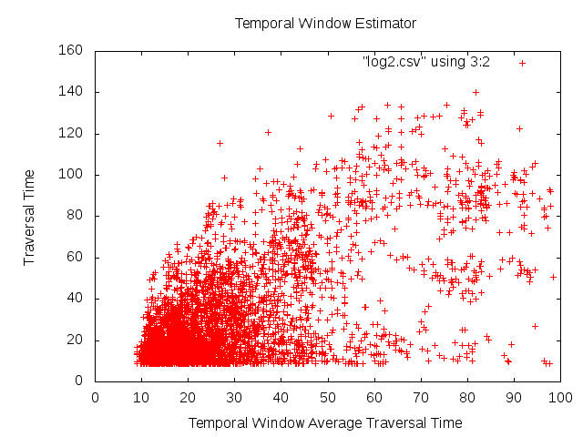
The real problem here is that cars don't load balance between their lanes, so the amount of traffic waiting on the lane that you happen to fall into largely determines your traversal time. As stated earlier, a car making a long sequence of planning choices through a large network of intersection will have no way of knowing what lane it will be in when it arrives at a given intersection, preventing us from using this information. Right now the temporal window's estimates fall on average within 15 seconds of the actual traversal time and this may not be too bad for the information we have access to. The next step would be to toss this data to Weka and see if any regression functions can do any better.
10/25/2010
An arff dataset compatible with Weka for the problem of estimating intersection traversal time is available here.
10/26/2010
Ran all of Weka's regression methods over the dataset (around 30). Best mean absolute error was 10.5 seconds by Bagging. This is basically the same as what I'm getting using the temporal window approach. The focus right now is to implement automatic lane changing in order to get some load balancing before the entrances to intersections which will hopefully lower the variance in traversal times.
11/7/2010
Work over the last couple focused on getting lane changing working. The idea is that lane changing will ideally help cars load-balance at the entrance to intersections, giving us more reliable estimates of their traversal times. Chiu had the lane changing code mostly hammered out but I've had to debug various sources of collisions over the past week. At this point everything seems to be working.
Experiments indicate that lane changing increases traffic throughput in a minor fashion -- a single intersection with 1500 cars/lane/hour showed a throughput of 2766 cars without lane changing and 2804 cars with lane changing -- for a 2.5% increase.
Most importantly, I reran the IM delay prediction regression experiments. The arff can be downloaded here. As we were expecting, lane changing does indeed make traversal time estimation more straightforwards. After running a variety of Weka's classifiers, the best of which was again the Bagging classifier, the best mean absolute error was 5.9 seconds. This is quite a reduction from the previous attempts 10.5 second error. This comes at the expense of a massive decision tree. Linear regression yields a MAE (mean absolute error) of 6.46 seconds with the all too simple function: 0.1403 * Longest Wait Time + 0.3019 * Temporal Window Estimate + 0.0706 * Total Active Vehicles + 1.4289 * Path Active Vehicles + 0.6733. I suspect for all intensive purposes this accuracy should be quite acceptable.
11/13/2010
Finished adding load balancing to the lane changing. This turned out to be far more complicated than originally expected for several reasons. First, the data structures which track a lane for lane changing were assume to track only a single lane, rather than multiple lanes needed for load balancing. After extending the necessary data structures it was then necessary to strike a balance between having cars switch into the correct lane for their turn direction (eg. left turning cars should enter the left lane) and the lane with least traffic. Ultimately this was accomplished using much ah-hoc logic. It would be a good idea in the future to come up with an equation which handles this nicely. The main bulk of the work was in debugging the lane changing apparatus, which has really become quite complicated at this point. The code is in need of refactoring. That point aside, the load balancing seems to be working correctly and the flow of traffic looks much more natural. A re-run of the traversal time estimation experiments yields a mean absolute error of 7.05 seconds which is not as good as before but not too bad. Associated dataset here. Additionally, the lane changing doesn't seem to slow the simulator down very much. A 500 simulated second run with traffic level 1000 took 4mins 43seconds with lane changing and 4min 37seconds without. This new load balancing also slightly improves the throughput of the system, with 1244 cars successfully traversing with lane changing and 1234 cars traversing without.
11/28/2010
Re-ran some experiments comparing the different navigation policies. This experiment consisted of a 2x2 grid which has (nearly) persistent traffic entering the top left and exiting the bottom right. Sporadic, heavy traffic enters the grid from either the bottom left or the top right. In all cases there is a way for the persistent traffic to avoid the sporadic traffic. What we are really interested in is the delay the persistent traffic encounters. The hypothesis is that the random algorithm will send only half of the cars along the correct route (the one avoiding the incoming traffic), which gives an opportunity for A* to route more cars along the correct route. The A* comes in two different flavors -- Full A* has all cars (including the traffic influx) use A* while partial A* only allows the persistent traffic to use A*, the influx traffic goes along a predetermined route. The optimal algorithm always routes traffic along pre-selected best route (eg the one which avoid the influx of traffic). The following table is the results of these algorithms compared along several different dimensions. The total throughput and total average delay are standard metrics. The favored metrics are equivalent except only computed over those cars which were members of the persistent traffic stream.| Method Type | Total Throughput (cars) | Favored Throughput (cars) | Total Avg Delay (sec) | Favored Avg Delay (sec) |
|---|---|---|---|---|
| Optimal | 1523 | 623 | 29.4395 | 11.9569 |
| Full A* | 1497 | 620 | 31.7281 | 14.8955 |
| Partial A* | 1531 | 623 | 30.5555 | 14.0394 |
| Random | 1506 | 614 | 36.1948 | 23.1803 |
12/1/2010
Two main changes to the simulator. First it was observed that cars turning right from the left lane would often turn into the rightmost lane of the target road rather than following their current lane (which would lead them into the leftmost lane of the target road). This was a result of drivers lane preferences which were determined by looking for the lane with the shortest distance from their current lane (hence the rightmost lane of the target road). Changing this to having drivers prefer to stay in their current lane or an adjacent lane results in a much more natural looking turn as well as higher throughput through intersections.
The second change was to make the favored traffic have a persistent source and destination and really become persistent. This means that when one source of sporadic traffic is incoming there remains a collisions free path through the intersection, but when the other source of traffic is incoming, our favored traffic must merge with it. Results from this new setup can be found here. To summarize, the results were as expected with the optimal algorithm taking the lead followed by the partial A* then full A*, and finally the random algorithm. There was one oddity in which the favored average delay of the optimal agent was higher than that of either A* agent. The differences where pretty small so I bet this falls within the bounds of experimental variations.
12/3/2010
The following image demonstrates Braess's Paradox within the simulator:

The "Persistent" traffic (purple line) enters at location "Source 1" and exits at "Destination 1." This traffic is employs temporal A* to path-plan which allows traffic to go through both intersection 1 and 2. The second type of traffic flows from Source 2 to Destination 2. It also uses A* to path plan which yields two feasible paths, Path A and Path B. Path B is the shorter and more direct path to the destination, but path A may be favored in cases in which Path B shows significant delays (typically before the entrance to intersection 3).
Braess's Paradox states that adding extra capacity to a network, when moving entities selfishly choose their route, can in some cases reduce the overall performance (Wikipedia). In order to prove this is a legitimate example of Braess's Paradox, we need to demonstrate the following:
- Removing the road in question improves overall network performance (in this case measured by throughput and delay).
- Cars are selfishly choosing their path.
To prove that cars are selfishly choosing paths, we examine the average time of the cars going from source 2 to destination 2 along both path A and path B. We argue adding the extra road creates path A which cars can selfishly follow at the expense of the overall network. The average traversal time from entering intersection 1 to reaching destination 2 for cars following Path B was 79.67 seconds while the average traversal for path A was only 60.33 seconds. This shows that the cars that choose path A are indeed acting greedily (by saving themselves travel time). At the same time they hurt the performance of the network at a whole.
Braess's Paradox is a pretty interesting thing in that it implies that in order to achieve optimal network flow, we must either create incentives for drivers to cooperate with each other or coerce them to do so by closing certain paths.
12/12/2010
As an addendum to the previous post, I should point out that in the optimal traffic routing scenario (when no cars take path A) the average traversal time of the traffic along path B is 52.35 seconds. Since the average traversal time of path A was 60.33 seconds, it seems that there would be no real incentive for the first car to take path A. Further experiments prove that this is not the case. When a very small stream of traffic, say 1% is routed along Path A, this traffic stream has an average traversal time of only 34.8644 seconds, far less than the average traversal time of Path B (55.9397 seconds). This means that the firsts cars to diverge really do have incentive to diverge. After the proverbial floodgates are opened many more quickly follow, leading to higher delays for all.
12/17/2010
When comparing the performance of AIM to that of traffic signals, AIM has in the past been much more efficient. Oddly, when using the scenario we have, optimal traffic signals prove to be nearly equal in performance to AIM (with cars navigating optimally). This is largely a result of the fact that there is only one point of possible conflict (eg the last intersection that both flows of traffic pass through). Interestingly, the delay imposed by the traffic signal at this single intersection was not large enough to distinguish AIM from traffic signals. I think this is because AIM incurs some delay through this intersection as well (due to traffic flows having slightly overlapping paths).
To differentiate traffic signals from AIM, we decided to add random traffic to the scenario. The idea behind this move was that most of the traffic signals along the way were simply staying green in one direction allowing the traffic flows to continuously pass. With small amounts of traffic needing to cross the intersection in different directions, traffic signals will be required to eventually give red lights to the main traffic flows. (Specifically this is implemented using a sum of wait times for each car along each different road into the intersection to determine which light should be green or red).
The normal flow of persistent traffic is 1500 cars/lane/hour. Adding 20 percent of this in random traffic per lane (eg 300 cars/lane/hour) to the scenario proved sufficient to differentiate traffic signals from AIM while preserving the relative ordering of results established earlier. Results can be viewed here or in the table below.
| Method Type | Total Throughput (cars) | Favored Throughput (cars) | Total Avg Delay (sec) | Favored Avg Delay (sec) |
|---|---|---|---|---|
| Optimal | 2281 (2271) | 942 (875) | 27.93 (50.35) | 19.46 (51.69) |
| Full A* | 2232 (2184) | 916 (842) | 33.59 (66.15) | 27.49 (66.3) |
| Partial A* | 2228 (2243) | 937 (881) | 34.46 (66.15) | 25.14 (55.08) |
| Random | 2094 (2170) | 912 (863) | 43.52 (57.07) | 41.7341 (59.1) |
| Non-adaptive | 2105 (2178) | 797 (866) | 59.33 (57.07) | 96.84 (66.15) |
Italicized numbers in the table represent the scenario run with traffic while non italicized numbers represent the scenario with AIM.
Interestingly AIM does roughly equal to traffic signals in terms of total throughput, but much better than signals in terms of average delay. This seems odd because it implies that it's possible to have a high throughput system with high delays. Perhaps further work should be done to understand the relationship between throughput and latency.
1/5/2011
I've implemented dynamic redirection of lanes. The basic idea is that one of the advantages of the AIM protocol is that the direction of the flow of traffic on lanes can be reversed quickly and efficiently in response to changes in the demand for different segments of road. The implementation required that cars be able to change lanes while going straight through an intersection (so they wouldn't end up driving into a closed lane). The implementation of dynamic lane changing first asks intersection managers to determine the demand for a given segment of road. The IMs know this because they keep track of the destination road of each car which has applied for a reservation to go through the intersection. If the demand of a certain road is greater than that of its dual (the road traveling in the opposite direction), lane(s) will be taken from the dual and added to the high demand road. Specific implementation details are more involved, but that is the basic idea.
To test the efficacy of dynamic lane changing we create a very simple test scenario in which flows of traffic alternate along a single road. For 100 seconds heavy traffic flows east along the road and then for the next 100 seconds heavy traffic flows west along the road. A total of six lanes exist which can be reconfigured as needed depending on the flow of traffic. (Current implementation requires that at least one lane exist in each direction -- so a max of 5 lanes can be opened in a single direction).

In this scenario, without dynamic lane changing the total throughput was 1239 cars over 1000 seconds versus 1335 cars with dynamic lane reversals. Additionally, the average delay of each car without lane reversals was 21.1815 seconds versus 2.7242 seconds with dynamic lane reversals.