Advanced Linear Algebra: Are you ready?
“I think that if a student can work through the problems slowly and understand most of the solutions, they would definitely be able to perform well in the course.” - Observation from former student in our graduate class
The primary purpose of this document is to facilitate the self-assessment of readiness for a first graduate level course on numerical linear algebra. It was created for our "Advanced Linear Algebra: Foundations to Frontiers" (ALAFF) [3] online resource, which is used by a Massive Open Online Course (MOOC) on edX by the same name. This resource is available for free from http://ulaff.net and the MOOC is free to auditors [4].
Most of the questions below involve concrete examples similar to what a learner may have seen in a first undergraduate course on linear algebra. To successfully complete a graduate level course on the subject, one must be able to master
Abstraction. This means that one must be able to take insights gained from manipulating concrete examples involving small matrices and vectors to extend to a general case.
Proofs. It does not suffice to be able to execute an algorithm in order to compute a result. Abstraction allows one to state general principles (theorems, lemmas, corollaries), which need to be proven true.
Algorithms. Numerical linear algebra is to a large degree about transforming theory into practical algorithms that are efficient and accurate in the presense of roundoff error.
Once you have solved a given problem, it is important to spend time not just with the answer, but also with our suggested full solution. It is from the solution that you get an idea of how abstraction generalizes a concrete example, how convincing arguments allow one to prove an assertion, and/or how an insight can be translated into an algorithm.
In addition to providing full solutions, we also discuss the relevance of the problem to a course in numerical linear algebra. For those who find that they need a refresher, we point to where related material can be found in "Linear Algebra: Foundations to Frontiers" (LAFF) [1], our online resource for a first undergraduate course in linear algebra, which can be taken (for free by auditors) as a MOOC on edX [2].
A course in graduate numerical linear algebra will have a heavy emphasis on mathematics and proofs. Some undergraduate courses in linear algebra also serve as a first introduction to proof techniques. Others do not. LAFF attempts to expose learners to the theorems and proofs that underlie the topic. Some may find they need more. It has been suggested that the MOOC "Introduction to Mathematical Thinking" by Keith Devlin, offered on Coursera, is a useful resource for this. (We have not personally examined that material.)
Additional information regarding our materials can be found at http://ulaff.net.
We hope this experience will help you assess what you need to do to get prepared!
Question 1.
Let \(v_0 , v_1 , \ldots , v_{k-1} \in \mathbb R^{n} \text{,}\) \(\alpha_0, \alpha_1, \ldots, \alpha_{k-1} \in \mathbb R \text{,}\) and \(L : \mathbb R^n \rightarrow \mathbb R^m \) be a linear transformation.
ALWAYS/SOMETIMES/NEVER: \(L( \sum_{i=0}^{k-1} \alpha_i v_i ) = \sum_{i=0}^{k-1} \alpha_i L( v_i ) \) for \(k \ge 0 \text{.}\)
Answer
ALWAYS
Now prove it!
Solution
\(L: \mathbb R^n \rightarrow \mathbb R^m \) is a linear transformation if and only if it satisfies the conditions
-
If \(\alpha \in \mathbb R \) and \(x \in \mathbb R^n \text{,}\) then \(L( \alpha x ) = \alpha L( x ) \text{.}\)
In other words, scaling a vector first and then transforming yields the same result as transforming the vector first and then scaling.
-
If \(x,y \in \mathbb R^n \text{,}\) then \(L( x + y ) = L( x ) + L( y ) \text{.}\)
In other words, adding two vectors first and then transforming yields the same result as transforming the vectors first and then adding.
We employ a proof by induction.
-
Base case: \(k = 0 \text{.}\)
We need to show that \(L( \sum_{i=0}^{0-1} \alpha_i v_i ) = \sum_{i=0}^{0-1} \alpha_i L( v_i ) \text{.}\)
\begin{equation*} \begin{array}{l} L( \sum_{i=0}^{0-1} \alpha_i v_i ) \\ ~~~ = ~~~~ \lt \mbox{ arithmetic } \gt \\ L( \sum_{i=0}^{-1} \alpha_i v_i ) \\ ~~~ = ~~~~ \lt \mbox{ summation over empty range. Here } 0 \mbox{ equals the zero vector } \gt \\ L( 0 ) \\ ~~~ = ~~~~ \lt \mbox{ a linear transformation maps } \mbox{the zero vector to a zero vector } \gt \\ 0 \\ ~~~ = ~~~~ \lt \mbox{ summation over empty range } \gt \\ \sum_{i=0}^{-1} \alpha_i L( v_i ) \\ ~~~ = ~~~~ \lt \mbox{ arithmetic } \gt \\ \sum_{i=0}^{0-1} \alpha_i L( v_i ) . \end{array} \end{equation*} -
Inductive step:
The Inductive Hypothesis (I.H.) assumes
\begin{equation*} L( \sum_{i=0}^{k-1} \alpha_i v_i ) = \sum_{i=0}^{k-1} \alpha_i L( v_i ). \end{equation*}for \(k = N \) with \(N \ge 0 \text{.}\) So, the Inductive Hypothesis is
\begin{equation*} L( \sum_{i=0}^{N-1} \alpha_i v_i ) = \sum_{i=0}^{N-1} \alpha_i L( v_i ). \end{equation*}Under this assumption we need to show that
\begin{equation*} L( \sum_{i=0}^{k-1} \alpha_i v_i ) = \sum_{i=0}^{k-1} \alpha_i L( v_i ). \end{equation*}for \(k = N+ 1 \text{.}\) In other words, we need to show that
\begin{equation*} L( \sum_{i=0}^{(N+1)-1} \alpha_i v_i ) = \sum_{i=0}^{(N+1)-1} \alpha_i L( v_i ). \end{equation*}Now,
\begin{equation*} \begin{array}[t]{l} L( \sum_{i=0}^{(N+1)-1} \alpha_i v_i ) \\ ~~~ = ~~~~ \lt \mbox{ arithmetic } \gt \\ L( \sum_{i=0}^{N} \alpha_i v_i ) \\ ~~~ = ~~~~ \lt \mbox{ split off last term } \gt \\ L( \sum_{i=0}^{N-1} \alpha_i v_i + \alpha_N v_N ) \\ ~~~ = ~~~~ \lt L \mbox{ is a linear transformation } \gt \\ L( \sum_{i=0}^{N-1} \alpha_i v_i ) + L( \alpha_N v_N ) \\ ~~~ = ~~~~ \lt L \mbox{ is a linear transformation } \gt \\ L( \sum_{i=0}^{N-1} \alpha_i v_i ) + \alpha_N L( v_N ) \\ ~~~ = ~~~~ \lt \mbox{ I.H. } \gt \\ \sum_{i=0}^{N-1} \alpha_i L( v_i ) + \alpha_N L( v_N ) \\ ~~~ = ~~~~ \lt \mbox{ add term to summation } \gt \\ \sum_{i=0}^{N} \alpha_i L( v_i ) \\ ~~~ = ~~~~ \lt \mbox{ arithmetic } \gt \\ \sum_{i=0}^{(N+1)-1} \alpha_i L( v_i ) . \end{array} \end{equation*} By the Principle of Mathematical Induction, the result holds. (This assertion is important, since it completes the reasoning. Alternatively, or in addition, you can state up front that you will use a proof by induction.)
Alternative solution
-
An alternative style of proof establishes that the expression simplifies to true via an "equivalence style" proof.
Base case: \(k = 0 \text{.}\)
We need to show that \(L( \sum_{i=0}^{0-1} \alpha_i v_i ) = \sum_{i=0}^{0-1} \alpha_i L( v_i ) \text{.}\)
\begin{equation*} \begin{array}{l} L( \sum_{i=0}^{0-1} \alpha_i v_i ) = \sum_{i=0}^{0-1} \alpha_i L( v_i ) \\ ~~~ \Leftrightarrow ~~~~ \lt \mbox{ arithmetic } \gt \\ L( \sum_{i=0}^{-1} \alpha_i v_i ) = \sum_{i=0}^{-1} \alpha_i L( v_i ) \\ ~~~ \Leftrightarrow ~~~~ \lt \mbox{ summation over empty range. Here } 0 \mbox{ equals the zero vector } \gt \\ L( 0 ) = 0 \\ ~~~ \Leftrightarrow ~~~~ \lt \mbox{ a linear transformation maps the zero } \mbox{vector to the zero vector } \gt \\ \mbox{true}. \end{array} \end{equation*} -
Inductive step:
Assume the Inductive Hypothesis (I.H.)
\begin{equation*} L( \sum_{i=0}^{k-1} \alpha_i v_i ) = \sum_{i=0}^{k-1} \alpha_i L( v_i ). \end{equation*}for \(k = N \) with \(N \ge 0 \text{.}\)
Under this assumption, we need to show that
\begin{equation*} L( \sum_{i=0}^{k-1} \alpha_i v_i ) = \sum_{i=0}^{k-1} \alpha_i L( v_i ). \end{equation*}for \(k = N+ 1 \text{.}\) In other words, we need to show that
\begin{equation*} L( \sum_{i=0}^{(N+1)-1} \alpha_i v_i ) = \sum_{i=0}^{(N+1)-1} \alpha_i L( v_i ). \end{equation*}Now,\begin{equation*} \begin{array}[t]{l} L( \sum_{i=0}^{(N+1)-1} \alpha_i v_i ) = \sum_{i=0}^{(N+1)-1} \alpha_i L( v_i ) \\ ~~~ \Leftrightarrow ~~~~ \lt \mbox{ arithmetic } \gt \\ L( \sum_{i=0}^{N} \alpha_i v_i ) = \sum_{i=0}^{N} \alpha_i L( v_i ) \\ ~~~ \Leftrightarrow ~~~~ \lt \mbox{ split off last term } \gt \\ L( \sum_{i=0}^{N-1} \alpha_i v_i + \alpha_N v_N ) = \sum_{i=0}^{N-1} \alpha_i L( v_i ) + \alpha_N L( v_N ) \\ ~~~ \Leftrightarrow ~~~~ \lt L \mbox{ is a linear transformation } \gt \\ L( \sum_{i=0}^{N-1} \alpha_i v_i ) + L( \alpha_N v_N ) = \sum_{i=0}^{N-1} \alpha_i L( v_i ) + \alpha_N L( v_N ) \\ ~~~ \Leftrightarrow ~~~~ \lt L \mbox{ is a linear transformation } \gt \\ L( \sum_{i=0}^{N-1} \alpha_i v_i ) + \alpha_N L( v_N ) = \sum_{i=0}^{N-1} \alpha_i L( v_i ) + \alpha_N L( v_N ) \\ ~~~ \Leftrightarrow ~~~~ \lt \mbox{ subtract equal term from both sides } \gt \\ L( \sum_{i=0}^{N-1} \alpha_i v_i ) = \sum_{i=0}^{N-1} \alpha_i L( v_i ) \\ ~~~ \Leftrightarrow ~~~~ \lt \mbox{ I.H.} \gt \\ \sum_{i=0}^{N-1} \alpha_i L( v_i ) = \sum_{i=0}^{N-1} \alpha_i L( v_i ) \\ ~~~ \Leftrightarrow ~~~~ \lt \mbox{ law of identity } \gt \\ \mbox{true}. \end{array} \end{equation*} By the Principle of Mathematical Induction, the result holds.
Either style of proof is acceptable. Some prefer even more informal reasoning. The important thing is that a correct, convincing argument is given.
Relevance
This question touches on a number of concepts in mathematics and linear algebra needed to master advanced topics. These include
Proof by induction. In linear algebra, we are typically interested in establishing results for all sizes of matrices or vectors. This often involves a proof by induction.
The summation quantifier. The summation quantifier allows us to specify summation over a variable number of elements in a set that has the summation operator defined on it.
The zero vector. The zero vector is the vector of appropriate size of all zeroes. It is denoted by \(0 \text{,}\) where the size of the vector is usually deduced from context.
Summation over the empty range. Summation over the empty range yields zero, which in the setting of this question means the zero vector.
Through the two solutions, we provide you are also exposed to proof styles that we use throughout ALAFF. Rather than making proofs as succinct as possible, we try to provide all intermediate steps, with justifications.
Resources
Simple proofs by induction, using the structured proof by induction demonstrated in the solution, can be found in Week 2 of LAFF.
Question 2.
Let the function \(f : \mathbb R^3 \rightarrow \mathbb R^2 \) be defined by
TRUE/FALSE: \(f \) is a linear transformation. Why?
-
If \(L \) is a linear transformation, there is a matrix that represents it. In other words, there exists a matrix \(A \) such that \(L( x ) = A x \text{.}\)
If you decided that the given \(f \) is a linear transformation, what is that matrix?
Answer
-
TRUE: \(f \) is a linear transformation.
Now prove it!
-
\(f( \left( \begin{array}{c} \chi_0 \\ \chi_1 \\ \chi_2 \end{array} \right) ) = \begin{array}[t]{c} \underbrace{ \left( \begin{array}{ r r r} 1 \amp 1 \amp 0\\ 1 \amp 0 \amp -1 \end{array} \right) } \\ A \end{array} \left( \begin{array}{c} \chi_0 \\ \chi_1 \\ \chi_2 \end{array} \right)\)
How did you find \(A \text{?}\)
Solution
-
We prove that the conditions for being a linear transformation, mentioned in the solution to Question 1, are met by
\begin{equation*} f( \left( \begin{array}{c} \chi_0 \\ \chi_1 \\ \chi_2 \end{array} \right) ) = \left( \begin{array}{c} \chi_0 + \chi_1 \\ \chi_0 - \chi_2 \end{array} \right) . \end{equation*}-
Let \(\alpha \in \mathbb R \) and \(x \in \mathbb R^n \) then
\begin{equation*} \begin{array}{l} f( \alpha x ) \\ ~~~ = ~~~~ \lt \mbox{ instantiate } \gt \\ f( \alpha \left( \begin{array}{c} \chi_0 \\ \chi_1 \\ \chi_2 \end{array} \right) ) \\ ~~~ = ~~~~ \lt \mbox{ scale the vector } \gt \\ f( \left( \begin{array}{c} \alpha \chi_0 \\ \alpha \chi_1 \\ \alpha \chi_2 \end{array} \right) ) \\ ~~~ = ~~~~ \lt \mbox{ definition of } f \gt \\ \left( \begin{array}{c} \alpha \chi_0 + \alpha \chi_1 \\ \alpha \chi_0 - \alpha \chi_2 \end{array} \right) \\ ~~~ = ~~~~ \lt \mbox{ factor out } \alpha \gt \\ \left( \begin{array}{c} \alpha ( \chi_0 + \chi_1 )\\ \alpha ( \chi_0 - \chi_2 ) \end{array} \right) \\ ~~~ = ~~~~ \lt \mbox{ scale the vector } \gt \\ \alpha \left( \begin{array}{c} \chi_0 + \chi_1 \\ \chi_0 - \chi_2 \end{array} \right)\\ ~~~ = ~~~~ \lt \mbox{ definition of } f \gt \\ \alpha f( \left( \begin{array}{c} \chi_0 \\ \chi_1 \\ \chi_2 \end{array} \right) ) \\ ~~~ = ~~~~ \lt \mbox{ instantiate } \gt \\ \alpha f( x ). \end{array} \end{equation*}Thus, scaling a vector first and then transforming yields the same result as transforming the vector first and then scaling.
-
Let \(x,y \in \mathbb R^n \) then
\begin{equation*} \begin{array}{l} f( x + y ) \\ ~~~ = ~~~~ \lt \mbox{ instantiate } \gt \\ f( \left( \begin{array}{c} \chi_0 \\ \chi_1 \\ \chi_2 \end{array} \right) + \left( \begin{array}{c} \psi_0 \\ \psi_1 \\ \psi_2 \end{array} \right) ) \\ ~~~ = ~~~~ \lt \mbox{ vector addition } \gt \\ f( \left( \begin{array}{c} \chi_0 + \psi_0 \\ \chi_1 + \psi_1 \\ \chi_2 + \psi_2 \end{array} \right) ) \\ ~~~ = ~~~~ \lt \mbox{ definition of } f \gt \\ \left( \begin{array}{c} ( \chi_0 + \psi_0 ) + ( \chi_1 + \psi_1 )\\ ( \chi_0 + \psi_0 ) - ( \chi_2 + \psi_2 ) \end{array} \right) \\ ~~~ = ~~~~ \lt \mbox{ associativity; communitivity } \gt \\ \left( \begin{array}{c} ( \chi_0 + \chi_1 ) + ( \psi_0 + \psi_1 )\\ ( \chi_0 - \chi_2 ) + ( \psi_0 - \psi_2 ) \end{array} \right) \\ ~~~ = ~~~~ \lt \mbox{ vector addition } \gt \\ \left( \begin{array}{c} \chi_0 + \chi_1 \\ \chi_0 - \chi_2 \end{array} \right) + \left( \begin{array}{c} \psi_0 + \psi_1 \\ \psi_0 - \psi_2 \end{array} \right) \\ ~~~ = ~~~~ \lt \mbox{ definition of } f \gt \\ f( \left( \begin{array}{c} \chi_0 \\ \chi_1 \\ \chi_2 \end{array} \right) ) + f ( \left( \begin{array}{c} \psi_0 \\ \psi_1 \\ \psi_2 \end{array} \right) ) \\ ~~~ = ~~~~ \lt \mbox{ instantiation } \gt \\ f( x ) + f ( y ) \end{array} \end{equation*}Hence, adding two vectors first and then transforming yields the same result as transforming the vectors first and then adding.
-
-
Some may be able to discover matrix \(A \) by examination. However, what we want you to remember is that for our linear transformation
\begin{equation*} \begin{array}{l} f( x ) \\ ~~~ = ~~~~ \lt \mbox{ instantiate } \gt \\ f( \left( \begin{array}{c} \chi_0 \\ \chi_1 \\ \chi_2 \end{array} \right) ) \\ ~~~ = ~~~~ \lt \mbox{ write vector as linear combination of standard basis vectors } \gt \\ f( \chi_0 \left( \begin{array}{c} 1 \\ 0 \\ 0 \end{array} \right) + \chi_1 \left( \begin{array}{c} 0 \\ 1 \\ 0 \end{array} \right) + \chi_2 \left( \begin{array}{c} 0 \\ 0 \\ 1 \end{array} \right) ) \\ ~~~ = ~~~~ \lt f \mbox{ is a linear transformation } \gt \\ \chi_0 f( \left( \begin{array}{c} 1 \\ 0 \\ 0 \end{array} \right) ) + \chi_1 f ( \left( \begin{array}{c} 0 \\ 1 \\ 0 \end{array} \right) ) + \chi_2 f ( \left( \begin{array}{c} 0 \\ 0 \\ 1 \end{array} \right) ) \\ ~~~ = ~~~~ \lt \mbox{ definition of } f \gt \\ \chi_0 \left( \begin{array}{c} 1 + 0 \\ 1 - 0 \end{array} \right) + \chi_1 \left( \begin{array}{c} 0 + 1 \\ 0 - 0 \end{array} \right) + \chi_2 \left( \begin{array}{c} 0 + 0 \\ 0 - 1 \\ \end{array} \right) \\ ~~~ = ~~~~ \lt \mbox{ arithmetic } \gt \\ \chi_0 \left( \begin{array}{r} 1 \\ 1 \end{array} \right) + \chi_1 \left( \begin{array}{r} 1 \\ 0 \end{array} \right) + \chi_2 \left( \begin{array}{r} 0 \\ - 1 \\ \end{array} \right) \\ ~~~ = ~~~~ \lt \mbox{ definition of matrix-vector multiplication } \gt \\ \left( \begin{array}{r r r} 1 \amp 1 \amp 0 \\ 1 \amp 0 \amp -1 \end{array} \right) \left( \begin{array}{c} \chi_0 \\ \chi_1 \\ \chi_2 \end{array} \right) \end{array} \end{equation*}More directly, if we partition \(A \) by columns
\begin{equation*} A = \left( \begin{array}{ c | c | c } a_0 \amp a_1 \amp a_2 \end{array} \right) \end{equation*}then
\begin{equation*} a_0 = f( \left( \begin{array}{c} 1 \\ 0 \\ 0 \end{array} \right) ), a_1 = f( \left( \begin{array}{c} 0 \\ 1 \\ 0 \end{array} \right) ), a_2 = f( \left( \begin{array}{c} 0 \\ 0 \\ 1 \end{array} \right) ). \end{equation*}Hence
\begin{equation*} A = \left( \begin{array}{r r r} 1 \amp 1 \amp 0 \\ 1 \amp 0 \amp -1 \end{array} \right) . \end{equation*}This captures the very important insight that the matrix captures the linear transformation by storing how the standard basis vectors are transformed by that linear transformation.
Relevance
The relation between linear transformations and matrices is central to linear algebra. It allows the theory of linear algebra to be linked to practical matrix computations, because matrices capture the action of linear transformations.
The exercise is relevant to advanced linear algebra in a number of ways.
It illustrates a minimal exposure to proofs that will be expected from learners at the start of the course.
-
It highlights that matrices first and foremost are objects that capture the "action" of a linear transformation.
Often, any two dimensional array of values is thought to be a matrix. However, not every two dimensional array captures an underlying linear transformation and hence it does not automatically qualify to be a matrix.
-
It emphasizes some of the notation that we will use in the notes for ALAFF:
Greek lower case letters are generally reserved for scalars.
Roman lower case letters are used to denote vectors.
Roman upper case letters are used for matrices.
It shows the level of detail that will be found in the solutions in the notes for ALAFF.
It illustrates how notation can capture the partitioning of a matrix by columns.
Resources
A learner who deduces from this exercise that they need a refresher on linear transformations may wish to spend some time with Week 2 and Week 3 of LAFF.
Question 3.
Let \(A \in \mathbb R^{m \times n} \) and \(x \in \mathbb R^n \text{.}\) How many floating point operations (flops) are required to compute the matrix-vector multiplication \(A x \text{?}\)
Answer
Approximately \(m n \) multiplies and \(m (n-1) \) adds, for a total of \(2 m n - m \) flops.
Solution
Let
Then
This exposes \(m n \) muiltiplications and \(m (n-1) \) additions, for a total of \(2 m n - m \) flops. We usually would state this as "approximately \(2 m n\) flops."
Alternative solution
A dot product \(x^T y \) with vectors of size \(n\) requires \(n \) multiplies and \(n-1 \) adds for \(2n-1 \) flops. A matrix-vector multiplication with an \(m \times n \) matrix requires \(m \) dot products with vectors of size \(n \text{,}\) for a total of \(m ( 2n-1) = 2mn - m\) flops.
Relevance
Matrix computations are at the core of many scientific computing and data science applications. Such applications often require substantial computational resources. Thus, reducing the cost (in time) of matrix computations is important, as is the ability to estimate that cost.
Resources
The cost of various linear algebra operations is discussed throughout LAFF. In particular, the video in Unit 1.4.1 of those notes is a place to start.
Question 4.
Compute \(\left( \begin{array}{r r r} 1 \amp -2 \amp 2 \\ -2 \amp 1 \amp -1\\ 2 \amp -1 \amp 1 \end{array} \right) \left( \begin{array}{r} 1 \\ 0 \\ -2 \end{array} \right) = \)
Compute \(\left( \begin{array}{r r r} 1 \amp -2 \amp 2 \\ -2 \amp 1 \amp -1\\ 2 \amp -1 \amp 1 \end{array} \right) \left( \begin{array}{r} -1 \\ 1 \\ 0 \end{array} \right) = \)
Compute \(\left( \begin{array}{r r r} 1 \amp -2 \amp 2 \\ -2 \amp 1 \amp -1\\ 2 \amp -1 \amp 1 \end{array} \right) \left( \begin{array}{r r} 1 \amp -1\\ 0 \amp 1 \\ -2 \amp 0 \end{array} \right) = \)
-
Why is matrix-matrix multiplication defined the way it is? In other words, if
\begin{equation*} A = \left( \begin{array}{c c c c} \alpha_{0,0} \amp \alpha_{0,1} \amp \cdots \amp \alpha_{0,k-1} \\ \alpha_{1,0} \amp \alpha_{1,1} \amp \cdots \amp \alpha_{1,k-1} \\ \vdots \amp \vdots \amp \amp \vdots \\ \alpha_{m-1,0} \amp \alpha_{m-1,1} \amp \cdots \amp \alpha_{m-1,k-1} \end{array} \right), B = \left( \begin{array}{c c c c} \beta_{0,0} \amp \beta_{0,1} \amp \cdots \amp \beta_{0,n-1} \\ \beta_{1,0} \amp \beta_{1,1} \amp \cdots \amp \beta_{1,n-1} \\ \vdots \amp \vdots \amp \amp \vdots \\ \beta_{k-1,0} \amp \beta_{k-1,1} \amp \cdots \amp \beta_{k-1,n-1} \end{array} \right), \end{equation*}and
\begin{equation*} C = \left( \begin{array}{c c c c} \gamma_{0,0} \amp \gamma_{0,1} \amp \cdots \amp \gamma_{0,n-1} \\ \gamma_{1,0} \amp \gamma_{1,1} \amp \cdots \amp \gamma_{1,n-1} \\ \vdots \amp \vdots \amp \amp \vdots \\ \gamma_{m-1,0} \amp \gamma_{m-1,1} \amp \cdots \amp \gamma_{m-1,n-1} \end{array} \right) \end{equation*}and \(C = A B \) then
\begin{equation*} \gamma_{i,j} = \sum_{p=0}^{k-1} \alpha_{i,p} \beta_{p,j}. \end{equation*}
Answer
\(\displaystyle \left( \begin{array}{r r r} 1 \amp -2 \amp 2 \\ -2 \amp 1 \amp -1\\ 2 \amp -1 \amp 1 \end{array} \right) \left( \begin{array}{r} 1 \\ 0 \\ -2 \end{array} \right) = \left( \begin{array}{r} -3 \\ 0 \\ 0 \end{array} \right) \)
\(\displaystyle \left( \begin{array}{r r r} 1 \amp -2 \amp 2 \\ -2 \amp 1 \amp -1\\ 2 \amp -1 \amp 1 \end{array} \right) \left( \begin{array}{r} -1 \\ 1 \\ 0 \end{array} \right) = \left( \begin{array}{r} -3 \\ 3 \\ -3 \end{array} \right) \)
\(\displaystyle \left( \begin{array}{r r r} 1 \amp -2 \amp 2 \\ -2 \amp 1 \amp -1\\ 2 \amp -1 \amp 1 \end{array} \right) \left( \begin{array}{r r} 1 \amp -1\\ 0 \amp 1 \\ -2 \amp 0 \end{array} \right) = \left( \begin{array}{r r} -3 \amp -3\\ 0 \amp 3 \\ 0 \amp -3 \end{array} \right) \)
-
Why is matrix-matrix multiplication defined the way it is?
\(C \) is matrix that represents the linear transformation that equals the composition of the linear transformations represented by \(A \) and \(B \text{.}\) That is, if \(L_A( y ) = A y \) and \(L_B ( x ) = B x \text{,}\) then \(L_C( x ) = L_A ( L_B ( x ) ) = C x \text{.}\)
Solution
\(\displaystyle \left( \begin{array}{r r r} 1 \amp -2 \amp 2 \\ -2 \amp 1 \amp -1\\ 2 \amp -1 \amp 1 \end{array} \right) \left( \begin{array}{r} 1 \\ 0 \\ -2 \end{array} \right) = \left( \begin{array}{r} -3 \\ 0 \\ 0 \end{array} \right) \)
\(\displaystyle \left( \begin{array}{r r r} 1 \amp -2 \amp 2 \\ -2 \amp 1 \amp -1\\ 2 \amp -1 \amp 1 \end{array} \right) \left( \begin{array}{r} -1 \\ 1 \\ 0 \end{array} \right) = \left( \begin{array}{r} -3 \\ 3 \\ -3 \end{array} \right) \)
-
\(\left( \begin{array}{r r r} 1 \amp -2 \amp 2 \\ -2 \amp 1 \amp -1\\ 2 \amp -1 \amp 1 \end{array} \right) \left( \begin{array}{r | r} 1 \amp -1\\ 0 \amp 1 \\ -2 \amp 0 \end{array} \right) = \left( \begin{array}{r | r} -3 \amp -3\\ 0 \amp 3 \\ 0 \amp -3 \end{array} \right) .\)
Notice that, given the computations in the first two parts, you should not have to perform any computations for this part. The reason is that if
\begin{equation*} C = A B, \end{equation*}and we partition \(C \) and \(B \) by rows,
\begin{equation*} C = \left( \begin{array}{c | c | c | c} c_0 \amp c_1 \amp \cdots \amp c_{n-1} \end{array} \right) \mbox{ and } B = \left( \begin{array}{c | c | c | c} b_0 \amp b_1 \amp \cdots \amp b_{n-1} \end{array} \right) , \end{equation*}then
\begin{equation*} \begin{array}{rcl} \left( \begin{array}{c | c | c | c} c_0 \amp c_1 \amp \cdots \amp c_{n-1} \end{array} \right) \amp = \amp A \left( \begin{array}{c | c | c | c} b_0 \amp b_1 \amp \cdots \amp b_{n-1} \end{array} \right) \\ \amp = \amp \left( \begin{array}{c | c | c | c} A b_0 \amp A b_1 \amp \cdots \amp A b_{n-1} \end{array} \right) . \end{array} \end{equation*}Thus, one can simply copy over the results from the first two parts into the columns of the result for this part.
-
Why is matrix-matrix multiplication defined the way it is?
An acceptable short answer would be to say that \(C \) equals the composition of the linear transformations represented by matrices \(A \) and \(B \text{,}\) which explains why \(C \) is computed the way it is.
-
The long answer:
Let \(L_A( x ) = A x \) and \(L_B = B x \) be the linear transformations that are represented by matrices \(A \) and \(B \text{,}\) respectively. It can be shown that the composition of \(L_A\) and \(L_B \text{,}\) defined by
\begin{equation*} L_C( x ) = L_A( L_B ( x ) ), \end{equation*}is a linear transformation.
Let \(C \) equal the matrix that represents \(L_C \text{,}\) \(e_j \) the \(j\)th standard basis vector (the column of the identity indexed with \(j \)), and partition
\begin{equation*} C = \left( \begin{array}{c | c | c | c} c_0 \amp c_1 \amp \cdots \amp c_{n-1} \end{array} \right) \mbox{ and } B = \left( \begin{array}{c | c | c | c} b_0 \amp b_1 \amp \cdots \amp b_{n-1} \end{array} \right) . \end{equation*}Then we know that
\begin{equation*} c_j = L_A( L_B( e_j ) ) = A( B e_j ) = A b_j. \end{equation*}Remembering how matrix-vector multiplication is computed, this means that
\begin{equation*} \gamma_{i,j} = \sum_{p=0}^{k-1} \alpha_{i,p} \beta_{p,j} = \widetilde a_i^T b_j. \end{equation*}This notation captures that element \(i,j \) of \(C \) equals the dot product of \(\widetilde a_i^T \text{,}\) the row of \(A \) indexed with \(i \text{,}\) and \(b_j \text{,}\) the column of \(B \) indexed with \(j \text{.}\)
Relevance
Almost every algorithm in linear algebra can be described as a sequence of matrix-matrix multiplications. Hence, understanding how to look at matrix-matrix multiplication in different ways is of utmost importance.
One way is the way you were likely first introduced to matrix-matrix multiplication, where each element of \(C \) is computed via a dot product of the appropriate row of \(A \) with the appropriate column of \(B \text{.}\)
Another is to compute columns of \(C \) as the product of \(A \) times the corresponding column of \(B \text{.}\) This is more directly related to why matrix-matrix multiplication is defined the way it is.
We will see more ways of looking at matrix-matrix multiplication in subsequent questions.
More generally, understanding how to multiply partitioned matrices is of central importance to the elegant, practical derivation and presentation of algorithms.
Resources
A learner who deduces from this exercise that they need a refresher on matrix-matrix multiplication may wish to spend some time with Week 4 and Week 5 of LAFF.
Question 5.
Let \(a_0 = \left( \begin{array}{r} -1 \\ 2 \\ 3 \end{array} \right) \) and \(b_0 = \left( \begin{array}{r} 1 \\ 0 \\ -2 \end{array} \right) \text{.}\) Compute \(a_0 b_0^T = \)
Let \(a_1 = \left( \begin{array}{r} 1 \\ -1 \\ 2 \end{array} \right)\) and \(b_1 = \left( \begin{array}{r} 0 \\ 1 \\ 2 \end{array} \right). \) Compute \(a_1 b_1^T =\)
Compute \(\left( \begin{array}{r r} -1 \amp 1 \\ 2 \amp -1 \\ 3 \amp 2 \end{array} \right) \left( \begin{array}{r r r} 1 \amp 0 \amp -2 \\ 0 \amp 1 \amp 2 \end{array} \right) =\)
Answer
- \begin{equation*} a_0 b_0^T = % \left( \begin{array}{r} % -1 \\ % 2 \\ % 3 % \end{array} \right) % \left( \begin{array}{r} % 1 \\ % 0 \\ % -2 % \end{array} \right)^T % = % \left( \begin{array}{r} % -1 \\ % 2 \\ % 3 % \end{array} \right) % \left( \begin{array}{r r r} % 1 \amp 0 \amp -2 % \end{array} \right) % = \left( \begin{array}{r r r} -1 \amp 0 \amp 2 \\ 2 \amp 0 \amp -4 \\ 3 \amp 0 \amp -6 \end{array} \right) \end{equation*}
- \begin{equation*} a_1 b_1^T = % \left( \begin{array}{r} % 1 \\ % -1 \\ % 2 % \end{array} \right) % \left( \begin{array}{r} % 0 \\ % 1 \\ % 2 % \end{array} \right)^T % = % \left( \begin{array}{r} % 1 \\ % -1 \\ % 2 % \end{array} \right) % \left( \begin{array}{r r r} % 0 \amp 1 \amp 2 % \end{array} \right) % = \left( \begin{array}{r r r} 0 \amp 1 \amp 2 \\ 0 \amp -1 \amp -2 \\ 0 \amp 2 \amp 4 \end{array} \right) \end{equation*}
\(\displaystyle \left( \begin{array}{r r} -1 \amp 1 \\ 2 \amp -1 \\ 3 \amp 2 \end{array} \right) \left( \begin{array}{r r r} 1 \amp 0 \amp -2 \\ 0 \amp 1 \amp 2 \end{array} \right) = \left( \begin{array}{r r r} -1 \amp 1 \amp 4 \\ 2 \amp -1 \amp -6 \\ 3 \amp 2 \amp -2 \end{array} \right) \)
Solution
When computing an outer product, we like to think of it as scaling rows
or scaling columns
This makes it easy to systematically compute the results:
- \begin{equation*} \begin{array}[t]{rcl} a_0 b_0^T \amp = \amp \left( \begin{array}{r} -1 \\ 2 \\ 3 \end{array} \right) \left( \begin{array}{r} 1 \\ 0 \\ -2 \end{array} \right)^T = \left( \begin{array}{r} -1 \\ 2 \\ 3 \end{array} \right) \left( \begin{array}{r r r} 1 \amp 0 \amp -2 \end{array} \right) \\ \amp = \amp \left( \begin{array}{r} (-1) \times \left( \begin{array}{r r r} 1 \amp 0 \amp -2 \end{array} \right) \\ \hline (2) \times \left( \begin{array}{r r r} 1 \amp 0 \amp -2 \end{array} \right) \\ \hline (3) \times \left( \begin{array}{r r r} 1 \amp 0 \amp -2 \end{array} \right) \end{array} \right) = \left( \begin{array}{r r r} -1 \amp 0 \amp 2 \\ 2 \amp 0 \amp -4 \\ 3 \amp 0 \amp -6 \end{array} \right) \end{array} \end{equation*}
- \begin{equation*} \begin{array}[t]{rcl} a_1 b_1^T \amp = \amp \left( \begin{array}{r} 1 \\ -1 \\ 2 \end{array} \right) \left( \begin{array}{r} 0 \\ 1 \\ 2 \end{array} \right)^T = \left( \begin{array}{r} 1 \\ -1 \\ 2 \end{array} \right) \left( \begin{array}{r | r | r} 0 \amp 1 \amp 2 \end{array} \right) \\ \amp = \amp \left( \begin{array}{r | r | r} (0) \times \left( \begin{array}{r} 1 \\ -1 \\ 2 \end{array} \right) \amp (1) \times \left( \begin{array}{r} 1 \\ -1 \\ 2 \end{array} \right) \amp (2) \times \left( \begin{array}{r} 1 \\ -1 \\ 2 \end{array} \right) \end{array} \right) \\ \amp = \amp \left( \begin{array}{r r r} 0 \amp 1 \amp 2 \\ 0 \amp -1 \amp -2 \\ 0 \amp 2 \amp 4 \end{array} \right) \end{array} \end{equation*}
-
Here there are two insights that make computing the result easier, given what has already been computed:
-
Notice that
\begin{equation*} \begin{array}{rcl} A B \amp =\amp \left( \begin{array}{c | c | c | c} a_0 \amp a_1 \amp \cdots \amp a_{k-1} \end{array} \right) \left( \begin{array}{c} b_0^T \\ \hline b_1^T \\ \hline \vdots \\ \hline b_{k-1}^T \end{array} \right)\\ \amp= \amp a_0 b_0^T + a_1 b_1^T + \cdots a_{k-1} b_{k-1}^T. \end{array} \end{equation*}Thus, we can use the results from the previous parts of this problem:
\begin{equation*} \begin{array}{l} \left( \begin{array}{r | r} -1 \amp 1 \\ 2 \amp -1 \\ 3 \amp 2 \end{array} \right) \left( \begin{array}{r r r} 1 \amp 0 \amp -2 \\ \hline 0 \amp 1 \amp 2 \end{array} \right) \\ ~~~ = \left( \begin{array}{r} -1 \\ 2 \\ 3 \end{array} \right) \left( \begin{array}{r r r} 1 \amp 0 \amp -2 \end{array} \right) + \left( \begin{array}{r} 1 \\ -1 \\ 2 \end{array} \right) \left( \begin{array}{r r r} 0 \amp 1 \amp 2 \end{array} \right) \\ ~~~ = \begin{array}[t]{c} \underbrace{ \left( \begin{array}{r r r} -1 \amp 0 \amp 2 \\ 2 \amp 0 \amp -4 \\ 3 \amp 0 \amp -6 \end{array} \right)} \\ \mbox{from first part} \end{array} + \begin{array}[t]{c} \underbrace{ \left( \begin{array}{r r r} 0 \amp 1 \amp 2 \\ 0 \amp -1 \amp -2 \\ 0 \amp 2 \amp 4 \end{array} \right) } \\ \mbox{from second part} \end{array} \\ ~~~ = \left( \begin{array}{r r r} -1 \amp 1 \amp 4 \\ 2 \amp -1 \amp -6 \\ 3 \amp 2 \amp -2 \end{array} \right). \end{array} \end{equation*}
-
Alternative solution
For the last part of the problem, we can alternatively use the insight that if
then
so that
Relevance
Again, we emphasize that understanding how to look at matrix-matrix multiplication in different ways is of utmost importance. In particular, viewing a matrix-matrix multiplication as the sum of a sequence of outer products (often called "rank-1 updates") is central to understanding important concepts, like expressing the Singular Value Decomposition (SVD) as the sum of a sequence of scaled outer products.
Resources
How to compute with matrices that have been "sliced and diced" (partitioned) as illustrated in the solution to this problem is discussed in great detail in Week 4 and Week 5 of LAFF.
Question 6.
Let \(L \in \mathbb R^{m \times m} \) be a nonsingular lower triangular matrix. Let us partition
where \(L_{TL} \) is square. Alternatively, partition
where \(L_{00} \) is square, \(l_{10}^T \) is a row vector, and \(\lambda_{11} \) is a scalar.
ALWAYS/SOMETIMES/NEVER: \(L_{TL}\) and \(L_{BR} \) are nonsingular.
-
ALWAYS/SOMETIMES/NEVER:
\begin{equation} L^{-1}= \left( \begin{array}{c | c} L_{00}^{-1} \amp 0 \\ \hline - l_{10}^T L_{00}^{-1} / \lambda_{11}\amp 1/\lambda_{11} \end{array} \right) \text{.}\label{linv-eqn}\tag{1} \end{equation} ALWAYS/SOMETIMES/NEVER: \(L^{-1} = \left( \begin{array}{c | c} L_{TL}^{-1} \amp 0 \\ \hline - L_{BR}^{-1} L_{BL} L_{TL}^{-1} \amp L_{BR}^{-1} \end{array} \right) \text{.}\)
Let \(L \) also be a unit lower triangular matrix (meaning it is lower triangular and all of its diagonal elements equal to \(1 \)).
ALWAYS/SOMETIMES/NEVER: \(L^{-1} \) is a unit lower triangular matrix.
ALWAYS: \(L_{TL}\) and \(L_{BR} \) are nonsingular.
ALWAYS: \(\left( \begin{array}{c | c} L_{00}^{-1} \amp 0 \\ \hline - l_{10}^T L_{00}^{-1} / \lambda_{11}\amp 1/\lambda_{11} \end{array} \right) \text{.}\)
ALWAYS: \(\left( \begin{array}{c | c} L_{TL}^{-1} \amp 0 \\ \hline - L_{BR}^{-1} L_{BL} L_{TL}^{-1} \amp L_{BR}^{-1} \end{array} \right) \text{.}\)
ALWAYS: \(L^{-1} \) is unit lower triangular.
Now prove it!
-
ALWAYS: \(L_{TL}\) and \(L_{BR} \) are nonsingular.
From an undergraduate level course you may remember that a lower triangular matrix is nonsingular if and only if none of its diagonal elements equal zero. Hence the proof goes something like
Clearly \(L_{TL} \) and \(L_{BR} \) are lower triangular.
Since \(L \) is nonsingular and lower triangular, none of its diagonal elements equal zero.
Hence none of its diagonal elements of \(L_{TL} \) and \(L_{BR} \) equal zero.
We conclude that \(L_{TL} \) and \(L_{BR} \) are nonsingular.
A careful reader may wonder what happens if \(L_{TL} \) or \(L_{BR} \) is \(0 \times 0 \text{.}\) This technical detail is solved by arguing that any \(0 \times 0 \) matrix \(A \) is nonsingular since the solution of \(A x = y \) is unique: only the empty vector (an vector with no elements) satisfies it.
-
ALWAYS: \(\left( \begin{array}{c | c} L_{00}^{-1} \amp 0 \\ \hline - l_{10}^T L_{00}^{-1} / \lambda_{11}\amp 1/\lambda_{11} \end{array} \right) \text{.}\)
One shows that \(B \) is the inverse of a matrix \(A \) by verifying that \(A B = I\) (the identity).
\begin{equation*} \begin{array}{l} \left( \begin{array}{c | c} L_{00} \amp 0 \\ \hline l_{10}^T \amp \lambda_{11} \end{array} \right) \left( \begin{array}{c | c} L_{00}^{-1} \amp 0 \\ \hline - l_{10}^T L_{00}^{-1} / \lambda_{11}\amp 1/\lambda_{11} \end{array} \right) ~~~ = ~~~~ \lt \mbox{ partitioned matrix-matrix multiplication } \gt \\ \left( \begin{array}{c | c} L_{00} L_{00}^{-1} \amp 0 \\ \hline l_{01}^T L_{00}^{-1} - \lambda_{11} l_{10}^T L_{00}^{-1} / \lambda_{11} \amp \lambda_{11} / \lambda_{11} \end{array} \right) \\ ~~~ = ~~~~ \lt C C^{-1} = I \gt \\ \left( \begin{array}{c | c} I \amp 0 \\ \hline 0 \amp 1 \end{array} \right) \\ ~~~ = ~~~~ \lt \mbox{ partitioned identity } \gt \\ I \end{array} \end{equation*}Here \(I \) equals an identity matrix "of appropriate size."
-
ALWAYS: \(\left( \begin{array}{c | c} L_{TL}^{-1} \amp 0 \\ \hline - L_{BR}^{-1} L_{BL} L_{TL}^{-1} \amp L_{BR}^{-1} \end{array} \right) \text{.}\)
\begin{equation*} \begin{array}{l} \left( \begin{array}{c | c} L_{TL} \amp 0 \\ \hline L_{BL} \amp L_{BR} \end{array} \right) \left( \begin{array}{c | c} L_{TL}^{-1} \amp 0 \\ \hline - L_{BR}^{-1} L_{BL} L_{TL}^{-1} \amp L_{BR}^{-1} \end{array} \right) \\ ~~~ = ~~~~ \lt \mbox{ partitioned matrix-matrix multiplication } \gt \\ \left( \begin{array}{c | c} L_{TL} L_{TL}^{-1} \amp 0 \\ \hline L_{BL} L_{TL}^{-1} - L_{BR} L_{BR}^{-1} L_{BL} L_{TL}^{-1} \amp L_{BR} L_{BR}^{-1} \end{array} \right) \\ ~~~ = ~~~~ \lt C C^{-1} = I \gt \\ \left( \begin{array}{c | c} I \amp 0 \\ \hline 0 \amp I \end{array} \right) \\ ~~~ = ~~~~ \lt \mbox{ partitioned identity } \gt \\ I \end{array} \end{equation*} -
Let \(L \) be unit lower triangular (meaning it is lower triangular and all of its diagonal elements equal \(1 \)).
ALWAYS: \(L^{-1} \) is unit lower triangular.
We employ a proof by induction. This time, we are going to look at a number of base cases, since the progression gives insight.
-
Base case 0: \(m = 0 \text{.}\)
This means \(L \) is a \(0 \times 0 \) unit lower triangular matrix. To make this case work, you have to accept that a \(0 \times 0 \) matrix is an identity matrix (and hence a unit lower triangular matrix). The argument is that an identity matrix is a matrix where all diagonal elements equal one. Since the \(0 \times 0 \) matrix has no elements, all its diagonal elements do equal one.
-
Base case 1: \(m = 1 \text{.}\) (Not really needed.)
This means \(L \) is a \(1 \times 1 \) unit lower triangular matrix. Hence \(L = 1 \text{.}\) Clearly, \(L^{-1} = 1 \text{,}\) which is a unit lower triangular matrix.
-
Base case 2: \(m = 2 \text{.}\) (Not really needed, but it provides some insight.)
This means \(L \) is a \(2 \times 2 \) unit lower triangular matrix. Hence
\begin{equation*} L = \left( \begin{array}{c| c} 1 \amp 0 \\ \hline \lambda_{10} \amp 1 \end{array} \right). \end{equation*}Using (1) with \(L_{00} = 1 \text{,}\) \(l_{10}^T = \lambda_{10} \text{,}\) and \(\lambda_{11} = 1 \text{,}\) we find that
\begin{equation*} L^{-1} = \left( \begin{array}{c | c} 1 \amp 0 \\ \hline -\lambda_{10} \amp 1 \end{array} \right), \end{equation*}which is a unit lower triangular matrix.
-
Inductive step:
Assume the Inductive Hypothesis (I.H.) that the inverses of all unit lower triangular matrices \(L \in \mathbb R^{m \times m} \) with \(m = k \text{,}\) where \(k \geq 0 \text{,}\) are unit lower triangular.
Under this assumption, we need to show that the inverse of any unit lower triangular matrix \(L \in \mathbb R^{m \times m} \) with \(m = k+1 \) is unit lower triangular.
Let \(L \in \mathbb R^{(k+1) \times (k+1)} \text{.}\) Partition
\begin{equation*} L = \left( \begin{array}{ c | c } L_{00} \amp 0 \\ \hline l_{10}^T \amp 1 \end{array} \right), \end{equation*}where \(L_{00} \in \mathbb R^{k \times k}\) is unit lower triangular and \(l_{10}^T \in \mathbb R^{1 \times k} \text{.}\) It can be easily checked that
\begin{equation*} L^{-1} = \left( \begin{array}{ c | c } L_{00}^{-1} \amp 0 \\ \hline - l_{10}^T L_{00}^{-1} \amp 1 \end{array} \right). \end{equation*}By the I.H., \(L_{00}^{-1} \) is unit lower triangular, and hence so is \(L^{-1} \text{.}\)
By the Principle of Mathematical Induction, the result holds.
-
Relevance
We keep hammering on this: understanding how to partition matrices and then multiply with partitioned matrices is key to being able to abstract away from concrete (and small) problems, and generalize to matrices of arbitrary size.
The notation we use, combined with the observation that
allows us to express an algorithm for inverting a nonsingular lower triangular matrix with what we call the FLAME notation that hides indexing into individual entries of a matrix:
This notation is used throughout ALAFF. The algorithm, as presented, illustrates the importance of allowing for the case where a matrix is \(0 \times 0 \text{.}\) In this example, \(L_{TL} \) (and hence \(L_{00} \)) is initially \(0 \times 0 \text{.}\)
Resources
In LAFF, we go to great lengths to help the learner extend their understanding gained from manipulating examples with small matrices and vectors to more general results and algorithms, using the partitioning of matrices and vectors (what we call "slicing and dicing" in that course). A prime example can be found in the discussion of an algorithm for Gaussian elimination, in Unit 6.2.5 of LAFF.
Question 7.
-
Solve
\begin{equation*} \begin{array}{r r r r} 2 \chi_0 + \amp \chi_1 + \amp \chi_2 = \amp 1 \\ -2 \chi_0 - \amp 2 \chi_1 + \amp \chi_2 = \amp -4 \\ 4 \chi_0 + \amp 4 \chi_1 + \amp \chi_2 = \amp 2 \\ \end{array} \end{equation*} Give the LU factorizaton of \(A = \left( \begin{array}{r r r} 2 \amp 1 \amp 1 \\ -2 \amp -2 \amp \phantom{-}1 \\ 4 \amp 4 \amp 1 \end{array} \right) \text{.}\)
Describe how one would use an LU factorization to solve \(A x = b \text{.}\)
-
Let
\begin{equation*} A = \left( \begin{array}{r r r} 2 \amp 1 \amp 1 \\ -2 \amp -2 \amp 1 \\ 4 \amp 4 \amp 1 \end{array} \right) \mbox{ and } b = \left( \begin{array}{r} 1 \\ -4 \\ 2 \end{array} \right). \end{equation*}TRUE/FALSE: \(b \) is in the column space of \(A \text{.}\)
Justify your answer.
Answer
\(\chi_0 = 2 \text{,}\) \(\chi_1 = -1 \text{,}\) and \(\chi_2 = -2 \text{.}\)
- \begin{equation*} \begin{array}[t]{c} \underbrace{ \left( \begin{array}{r r r} 2 \amp 1 \amp 1 \\ -2 \amp -2 \amp 1 \\ 4 \amp 4 \amp 1 \end{array} \right) } \\ A \end{array} = \begin{array}[t]{c} \underbrace{ \left( \begin{array}{r r r} 1 \amp 0 \amp 0 \\ -1 \amp 1 \amp 0 \\ 2 \amp -2 \amp 1 \end{array} \right) } \\ L \end{array} \begin{array}[t]{c} \underbrace{ \left( \begin{array}{r r r} 2 \amp 1 \amp 1 \\ 0 \amp -1 \amp 2 \\ 0 \amp 0 \amp 3 \end{array} \right) } \\ U \end{array} \end{equation*}
See "Solution."
-
TRUE
Now prove it.
Solution
-
\begin{equation*} \begin{array}{r r r r} 2 \chi_0 + \amp \chi_1 + \amp \chi_2 = \amp 1 \\ -2 \chi_0 - \amp 2 \chi_1 + \amp \chi_2 = \amp -4 \\ 4 \chi_0 + \amp 4 \chi_1 + \amp \chi_2 = \amp 2 \\ \end{array} \end{equation*}
can be represented by the appended system
\begin{equation*} \left( \begin{array}{r r r | r} 2 \amp 1 \amp \phantom{-}1 \amp 1 \\ -2 \amp -2 \amp 1 \amp -4 \\ 4 \amp 4 \amp 1 \amp 2 \\ \end{array} \right). \end{equation*}Subtracting \(-1 \) times the first row from the second row and subtracting \(2 \) times the first row from the third row yields
\begin{equation*} \left( \begin{array}{r r r | r} 2 \amp 1 \amp 1 \amp 1 \\ 0 \amp -1 \amp 2 \amp -3 \\ 0 \amp 2 \amp -1 \amp 0 \\ \end{array} \right). \end{equation*}Subtracting \(-2 \) times the second row from the third row yields
\begin{equation*} \left( \begin{array}{r r r | r} 2 \amp 1 \amp 1 \amp 1 \\ 0 \amp -1 \amp 2 \amp -3 \\ 0 \amp 0 \amp 3 \amp -6 \\ \end{array} \right). \end{equation*}This translates to
\begin{equation*} \begin{array}{r r r r} 2 \chi_0 + \amp \chi_1 + \amp \chi_2 = \amp 1 \\ \amp - \chi_1 + \amp 2 \chi_2 = \amp -3 \\ \amp \amp 3 \chi_2 = \amp -6 \end{array} \end{equation*}Solving this upper triangular system yields \(\chi_2 = -2 \text{,}\) \(\chi_1 = -1 \text{,}\) and \(\chi_0 = 2 \text{.}\)
-
The LU factorization can be read off from the above "Gaussian elimination" process for reducing the system of linear equations to an upper triangular system of linear equations:
\begin{equation*} \begin{array}[t]{c} \underbrace{ \left( \begin{array}{r r r} 2 \amp 1 \amp 1 \\ -2 \amp -2 \amp 1 \\ 4 \amp 4 \amp 1 \end{array} \right) } \\ A \end{array} = \begin{array}[t]{c} \underbrace{ \left( \begin{array}{r r r} 1 \amp 0 \amp 0 \\ -1 \amp 1 \amp 0 \\ 2 \amp -2 \amp 1 \end{array} \right) } \\ L \end{array} \begin{array}[t]{c} \underbrace{ \left( \begin{array}{r r r} 2 \amp 1 \amp 1 \\ 0 \amp -1 \amp 2 \\ 0 \amp 0 \amp 3 \end{array} \right) } \\ U \end{array} \end{equation*} -
If \(A = L U \) then
\begin{equation*} A x = b \end{equation*}can be rewritten as
\begin{equation*} ( L U ) x = b . \end{equation*}Associativity of multiplication yields
\begin{equation*} L ( U x ) = b . \end{equation*}If we introduce the variable \(z = U x \) we get that
\begin{equation*} L z = b. \end{equation*}Thus, we can first solve the lower triangular system \(L z = b \) and then \(U x = z \text{,}\) which yields the desired solution \(x \text{.}\)
-
TRUE
We saw in the first part of this question that
\begin{equation*} x = \left( \begin{array}{r} 2 \\ -1 \\ -2 \end{array} \right) \end{equation*}solves \(A x = b \text{.}\) Hence \(b \) can be written as a linear combination of the columns of \(A \text{:}\)
\begin{equation*} \left( \begin{array}{r} 1 \\ -4 \\ 2 \end{array} \right) = (2) \left( \begin{array}{r} 2 \\ -2 \\ 4 \end{array} \right) + (-1) \left( \begin{array}{r} 1 \\ -2 \\ 4 \end{array} \right) + (-2) \left( \begin{array}{r} 1 \\ 1 \\ 1 \end{array} \right) \end{equation*}which means that \(b \) is in the column space of \(A \text{.}\)
Relevance
Solving linear systems is fundamental to scientific computing and data sciences. While (Gaussian) elimination is a technique taught already in high school algebra, it is by presenting it as a factorization of matrices that it can be made systematic and implemented. Viewing it this way is also fundamental to being able to analyze how computer arithmetic and algorithms interact, which is at the core of the numerical linear algebra covered in an advanced linear algebra course.
Solving "dense" linear systems is also a convenient vehicle for discussing how to achieve high performance on current computer architectures.
Resources
In Week 6 and Week 7 of LAFF, solving linear systems via Gaussian elimination is linked to LU factorization.
Question 8.
Consider
TRUE/FALSE: \(A \) has linearly independent columns.
Reduce the appended system \(\left( \begin{array}{ c | c} A \amp b \end{array} \right)\) to row echelon form.
In the row echelon form (above): Identify the pivot(s). Identify the free variable(s). Identify the dependent variable(s).
Compute a specific solution.
Compute a basis for the null space of \(A \text{.}\)
TRUE/FALSE: This matrix is singular.
Give a formula for the general solution.
Give a basis for the column space of \(A \text{.}\)
Give a basis for the row space of \(A \text{.}\)
What is the rank of the matrix?
Identify two linearly independent vectors that are orthogonal to the null space of \(A \text{.}\)
Answer
FALSE: \(A \) does not have linearly independent columns.
- \begin{equation*} \left(\begin{array}{r r r | r} -1 \amp -3 \amp -3 \amp -5 \\ 0 \amp 4 \amp 4 \amp 8\\ 0 \amp 0 \amp 0 \amp 0 \end{array}\right) \end{equation*}
-
In the row echelon form (above): Identify the pivot(s). Identify the free variable(s). Identify the dependent variable(s).
\begin{equation*} \left(\begin{array}{r r r | r} {\color{red} {-1}} \amp -3 \amp -3 \amp -5 \\ 0 \amp {\color{red} 4} \amp 4 \amp 8\\ 0 \amp 0 \amp 0 \amp 0 \end{array}\right) \end{equation*}Pivots are highlighted in red. Free variable: \(\chi_2 \text{.}\) Dependent variables: \(\chi_0 \) and \(\chi_1 \text{.}\)
-
Compute a specific solution.
Solution:\(\left( \begin{array}{r} -1 \\ 2 \\ 0 \end{array}\right)\)
-
Compute a basis for the null space of \(A \text{.}\)
Solution:
\begin{equation*} \left( \begin{array}{r} 0 \\ -1 \\ 1 \end{array}\right). \end{equation*} TRUE: This matrix is singular.
-
Give a formula for the general solution.
\(\left( \begin{array}{c} -1 \\ 2 \\ 0 \end{array}\right) + \beta \left( \begin{array}{c} 0 \\ -1 \\ 1 \end{array}\right)\) (This is only one of many possible answers.)
-
Give a basis for the column space of \(A \text{.}\)
\begin{equation*} \left\{ \left(\begin{array}{r r r | r} -1 \\ -1 \\ -2 \end{array}\right) , \left(\begin{array}{r r r | r} -3 \\ 1 \\ -2 \end{array}\right) \right\}. \end{equation*} -
Give a basis for the row space of \(A \text{.}\)
\begin{equation*} \left\{ \left(\begin{array}{r r r | r} -1 \\ -3 \\ -3 \end{array}\right) , \left(\begin{array}{r r r | r} 0 \\ 4 \\ 4 \end{array}\right) \right\}. \end{equation*}The first two rows of original matrix is also a correct answer in this case, since no pivoting was required while reducing the matrix to row echelon form.
-
What is the rank of the matrix?
\(2 \) (the number of linearly independent columns).
-
Identify two linearly independent vectors that are orthogonal to the null space of \(A \text{.}\)
The vectors that form a basis for the row space can be used for this.
Solution
-
FALSE: \(A \) does not have linearly independent columns.
You may see this immediately "by inspection", since the second and third columns are equal, or you may deduce this after doing some of the remaining parts of this question.
-
Reduce the appended system \(\left( \begin{array}{ c | c} A \amp b \end{array} \right)\) to row echelon form.
\begin{equation*} \begin{array}{rcl} \left(\begin{array}{r r r | r} -1 \amp -3 \amp -3 \amp -5 \\ -1 \amp 1 \amp 1 \amp 3\\ -2 \amp -2 \amp -2 \amp -2 \end{array}\right) \amp \longrightarrow \amp \left(\begin{array}{r r r | r} -1 \amp -3 \amp -3 \amp -5 \\ 0 \amp 4 \amp 4 \amp 8\\ 0 \amp 4 \amp 4 \amp 8 \end{array}\right) \\ \amp \longrightarrow \amp \left(\begin{array}{r r r | r} -1 \amp -3 \amp -3 \amp -5 \\ 0 \amp 4 \amp 4 \amp 8\\ 0 \amp 0 \amp 0 \amp 0 \end{array}\right) \end{array} \end{equation*} -
In the row echelon form (above): Identify the pivot(s). Identify the free variable(s). Identify the dependent variable(s).
\begin{equation*} \left(\begin{array}{r r r | r} {\color{red} {-1}} \amp -3 \amp -3 \amp -5 \\ 0 \amp {\color{red} 4} \amp 4 \amp 8\\ 0 \amp 0 \amp 0 \amp 0 \end{array}\right) \end{equation*}Pivots are highlighted in red. Free variable: \(\chi_2 \text{.}\) Dependent variables: \(\chi_0 \) and \(\chi_1 \text{.}\)
-
Compute a specific solution.
\begin{equation*} \left(\begin{array}{r r r} {-1} \amp -3 \amp -3 \\ 0 \amp {4} \amp 4 \end{array}\right) \left( \begin{array}{c} ? \\ ?\\ 0 \end{array}\right) = \left(\begin{array}{r} -5 \\ 8\end{array}\right), \end{equation*}where \(? \) is to be determined, yields
\(\displaystyle \chi_1 = 2 \)
\(-\chi_0 - 3 (2) = -5 \) so that \(\chi_0 = -1 \text{.}\)
Solution:\(\left( \begin{array}{r} -1 \\ 2 \\ 0 \end{array}\right)\)
-
Compute a basis for the null space of \(A \text{.}\)
\begin{equation*} \left(\begin{array}{r r r} {-1} \amp -3 \amp -3 \\ 0 \amp {4} \amp 4 \end{array}\right) \left( \begin{array}{c} ? \\ ? \\ 1 \end{array}\right) = \left(\begin{array}{r} 0 \\ 0\end{array}\right) \end{equation*}means
\(4 \chi_1 + 4 = 0 \) and hence \(\chi_1 = -1 \text{.}\)
\(-\chi_0 - 3 (-1) - 3 = 0 \) so that \(\chi_0 = 0 \text{.}\)
Solution:
\begin{equation*} \left( \begin{array}{r} 0 \\ -1 \\ 1 \end{array}\right). \end{equation*}You may have solved this by examination, which is fine.
-
TRUE: This matrix is singular.
There are a number of ways of justiifying this answer with what we have answered for this question so far:
The number of pivots is less than the number of columns of the matrix.
There are free variables.
There is a nontrivial vector in the null space.
\(A x = 0 \) has a nontrivial solution.
-
Give a formula for the general solution.
\begin{equation*} \left( \begin{array}{c} -1 \\ 2 \\ 0 \end{array}\right) + \beta \left( \begin{array}{c} 0 \\ -1 \\ 1 \end{array}\right) \end{equation*}This is only one of many possible answers that expresses the set of solutions.
-
Give a basis for the column space of \(A \text{.}\)
\begin{equation*} \left\{ \left(\begin{array}{r r r | r} -1 \\ -1 \\ -2 \end{array}\right) , \left(\begin{array}{r r r | r} -3 \\ 1 \\ -2 \end{array}\right) \right\}. \end{equation*} -
Give a basis for the row space of \(A \text{.}\)
\begin{equation*} \left\{ \left(\begin{array}{r r r | r} -1 \\ -3 \\ -3 \end{array}\right) , \left(\begin{array}{r r r | r} 0 \\ 4 \\ 4 \end{array}\right) \right\}. \end{equation*}The first two rows of original matrix is also a correct answer in this case, since no pivoting was required while reducing the matrix to row echelon form.
-
What is the rank of the matrix?
\(2 \) (the number of linearly independent columns).
-
Identify two linearly independent vectors that are orthogonal to the null space of \(A \text{.}\)
The vectors that are a basis for the row space can be used for this.
Relevance
Many questions in linear algebra have an infinite number of answers. For example, the answer to "for which right-hand side vectors \(b \) does \(A x = b \) have a solution?" typically is a set of vectors that has not only an infinite number of members, but an uncountable number of members. Describing that set with only a finite number of vectors (the basis for the subspace that equals the set) allows one to concisely answer various questions. Thus, the notions vector subspace, basis for the subspace, and dimension of the subspace are of central importance to linear algebra.
Another imporant concept touched upon in this question is the concept of the four fundamental spaces: the column, null, row, and left-null spaces. (The question refers to three out of four of these.) These can be visualized as
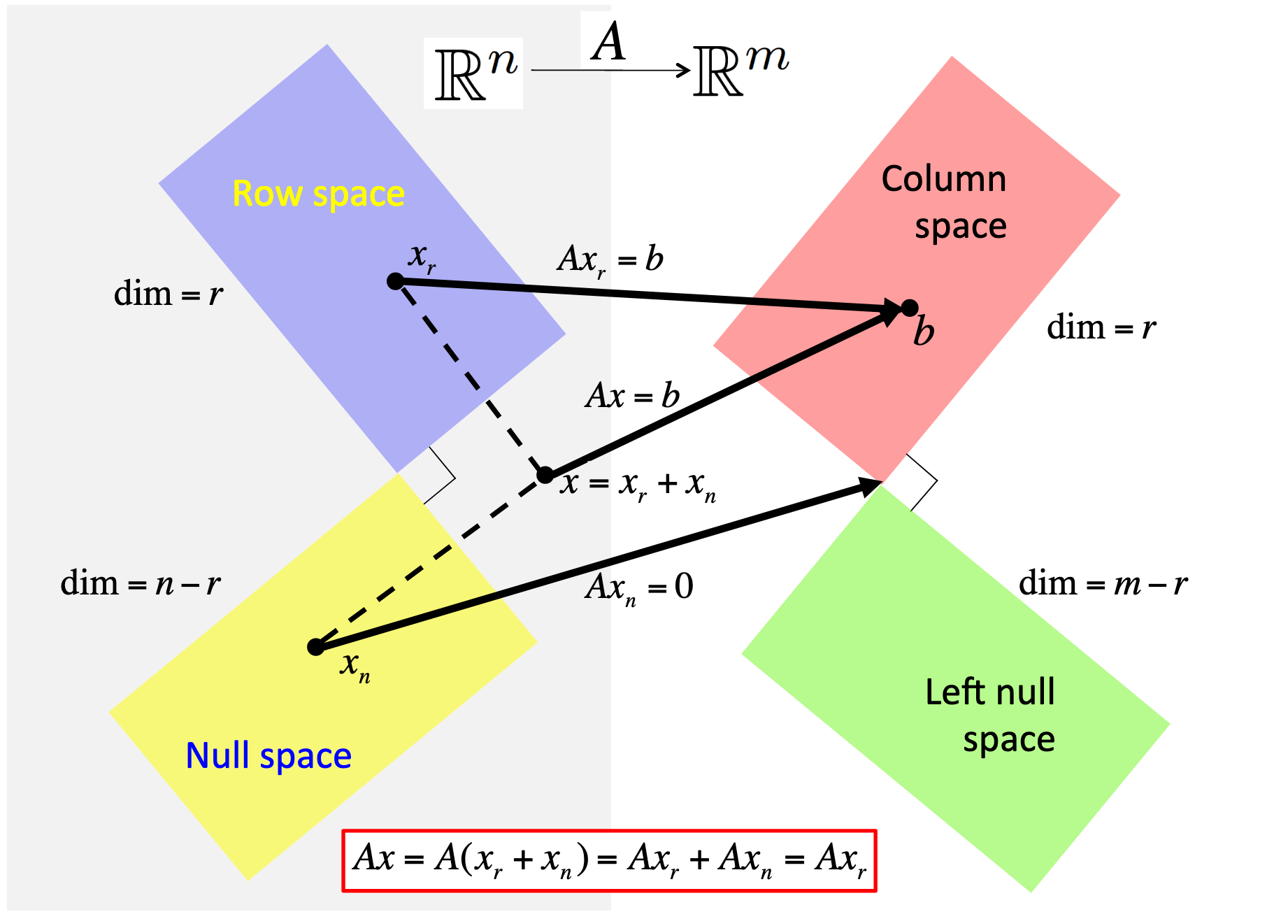
The process that reduces an appended matrix to row echelon form is actually not of much practical value. The reason is that when computer arithmetic is employed, roundoff error is incurred and hence the notion of a zero, central to interpreting the row echelon form, is fuzzy. In numerical linear algebra, we will employ other techiques for identifying bases for the four fundamental subspaces.
Resources
Week 9 and Week 10 of LAFF discuss the concepts and techniques relevant to this question.
Question 9.
Let \(A \in \mathbb R^{m \times n} \text{.}\)
ALWAYS/SOMETIMES/NEVER: The row space of \(A \) is orthogonal to the null space of \(A \text{.}\)
ALWAYS
Now prove it!
Vector \(u \) is in the row space of \(A \) if and only if there exists a vector \(x \) such that \(u = A^T x \text{.}\)
Vector \(v \) is in the null space of \(A \) if and only if \(A v = 0 \text{.}\)
Two vector spaces are orthogonal if and only if all vectors in one space are orthogonal to all vectors in the other space.
Let \(u \) be an arbitrary vector in the row space of \(A \) and \(v \) an arbitrary vector in the null space of \(A \text{.}\) Then
Relevance
The four fundamental spaces, and the orthogonality of those spaces, is fundamental to the theory and practice of linear algebra. Proving orthogonality of vectors and spaces is thus central to the topics?.
Resources
Week 10 of LAFF discusses vector spaces and orthogonality.
Question 10.
Consider
-
Give the best approximate solution (in the linear least squares sense) to
\begin{equation*} A x \approx b. \end{equation*} What is the orthogonal projection of \(b \) onto the column space of \(A \text{?}\)
TRUE/FALSE: \(b \) in the column space of \(A \text{.}\)
Answer
\(\displaystyle \left(\begin{array}{r} 2\\ -1 \end{array}\right). \)
\(\displaystyle \left(\begin{array}{r} -2\\ 5 \\ 3 \end{array}\right).\)
-
FALSE
Why?
Solution
-
Given a matrix \(A \in \mathbb R^{m \times n} \) and vector \(b \in \mathbb R^m \text{,}\) the approximate solution, in the linear least squares sense, to \(A x = b \) equals a vector that minimizes
\begin{equation*} \min_{x \in \mathbb R^n} \| b - A x \|_2, \end{equation*}the Euclidean length of the difference between \(b\) and \(A x \text{.}\) If the columns of \(A \) are linearly independent, the solution is unique. It is not hard to prove that the given \(A \) has linearly independent columns.
A straight forward way of computing this best approximate solution is to solve the normal equations: \(A^T A x = A^T b.\) Thus, we solve
\begin{equation*} \left( \begin{array}{r r} -1 \amp 0 \\ 2 \amp -1 \\ 2 \amp 1 \end{array} \right)^T \left( \begin{array}{r r} -1 \amp 0 \\ 2 \amp -1 \\ 2 \amp 1 \end{array} \right) \left( \begin{array}{c} \chi_0 \\ \chi_1 \end{array} \right) = \left( \begin{array}{r r} -1 \amp 0 \\ 2 \amp -1 \\ 2 \amp 1 \end{array} \right)^T \left( \begin{array}{r} 2 \\ 6 \\ 4 \end{array} \right), \end{equation*}which simplifies to
\begin{equation*} \left( \begin{array}{r r} 9 \amp 0 \\ 0 \amp 2 \end{array} \right) \left( \begin{array}{c} \chi_0 \\ \chi_1 \end{array} \right) = \left(\begin{array}{r} 18\\ -2 \end{array}\right), \end{equation*}(it is a happy coincidence that here \(A^T A \) is diagonal) and finally yields the solution
\begin{equation*} \left( \begin{array}{c} \chi_0 \\ \chi_1 \end{array} \right) = \left(\begin{array}{r} 2\\ -1 \end{array}\right). \end{equation*}We notice that \(x = ( A^T A )^{-1} A^T b \text{.}\) The matrix \(( A^T A)^{-1} A^T \) is known as the (left) pseudo-inverse of matrix \(A \text{.}\)
-
The orthogonal projection of \(b \) onto the column space of \(A \) is the vector \(A x \) that minimizes
\begin{equation*} \min_{x \in \mathbb R^n} \| b - A x \|_2. \end{equation*}Since we have computed the \(x \) that minimizes this in the last part of this question, the answer is
\begin{equation*} \begin{array}{rcl} A x \amp = \amp A \begin{array}[t]{c} \underbrace{( A^T A )^{-1} A^T b}\\ x \end{array} = \left( \begin{array}{r r} -1 \amp 0 \\ 2 \amp -1 \\ 2 \amp 1 \end{array} \right) \left( \begin{array}{c} \chi_0 \\ \chi_1 \end{array} \right) \\ \amp = \amp \left( \begin{array}{r r} -1 \amp 0 \\ 2 \amp -1 \\ 2 \amp 1 \end{array} \right) \left(\begin{array}{r} 2\\ -1 \end{array}\right) = \left(\begin{array}{r} -2\\ 5 \\ 3 \end{array}\right). \end{array} \end{equation*} Since the orthogonal projection of \(b \) onto the column space of \(A \) is not equal to \(b\text{,}\) we conclude that \(b \) is not in the column space of \(A \text{.}\)
Relevance
Solving linear least squares problems is of central importance to data sciences and scientific computing. It is synonymous with "linear regression."
In our example, the matrix happens to have orthogonal columns, and as a result \(A^T A \) is diagonal. More generally, when \(A \) has linearly independent columns, \(A^T A \) is symmetric positive definite (SPD). This allows the solution of \(A^T A x = A^T b\) to utilize a variant of LU factorization known as the Cholesky factorization that takes advantage of symmetry to reduce the cost of finding the solution. Reducing the cost (in time) is important since in data sciences and scientific computing one often wants to solve very large problems.
The method of normal equations is the simplest way for solving linear least squares problems. In the practical setting discussed in advanced linear algebra, one finds out that computer arithmetic, which invariably introduces round off error, can lead to an amplification of error when the columns of matrix \(A \) are almost linearly dependent. For such a matrix, it may be necessary to use other methods to obtain an accurate solution.
Resources
Week 10 of LAFF discusses the method of normal equations and how to use it to solve the linear least squares problem.
Question 11.
Let \(A = \left(\begin{array}{rrr} 1 \amp 0 \\ 1 \amp 1 \\ 0 \amp 1 \\ 0 \amp 1 \end{array}\right)\text{.}\)
Compute an orthonormal basis for the space spanned by the columns of \(A \text{.}\) No need to simplify expressions.
Give the QR factorization of matrix \(A \text{,}\) \(A = Q R \text{.}\)
Answer
Orthonormal basis: \(\frac{1}{\sqrt{2}} \left(\begin{array}{r} 1 \\ 1 \\ 0 \\ 0 \end{array}\right) \mbox{ and } \frac{\sqrt{2}}{ \sqrt{5} } \left(\begin{array}{rrr} -\frac{1}{2} \\ \frac{1}{2} \\ 1 \\ 1 \end{array}\right) \text{.}\)
-
For our example, the QR factorization of the matrix is given by
\begin{equation*} \begin{array}[t]{c} \underbrace{ \left( \begin{array}{c | c} a_0 \amp a_1 \end{array} \right) } \\ A \end{array} = \begin{array}[t]{c} \underbrace{ \left( \begin{array}{c | c} q_0 \amp q_1 \end{array} \right) } \\ Q \end{array} \begin{array}[t]{c} \underbrace{ \left( \begin{array}{c | c} \rho_{0,0} \amp \rho_{0,1} \\ \hline 0 \amp \rho_{1,1} \\ \end{array} \right) } \\ R \end{array} \end{equation*}Thus
\begin{equation*} \left(\begin{array}{r| rr} 1 \amp 0 \\ 1 \amp 1 \\ 0 \amp 1 \\ 0 \amp 1 \end{array}\right) = \left( \begin{array}{ c | c } \frac{1}{\sqrt{2}} \left(\begin{array}{r} 1 \\ 1 \\ 0 \\ 0 \end{array}\right) \amp \frac{\sqrt{2}}{ \sqrt{5} } \left(\begin{array}{rrr} -\frac{1}{2} \\ \frac{1}{2} \\ 1 \\ 1 \end{array}\right) \end{array} \right) \left( \begin{array}{ c | c } \sqrt{2} \amp 1/\sqrt{2} \\ \hline 0 \amp \frac{\sqrt{5}}{\sqrt{2}} \end{array} \right) . \end{equation*}
Solution
-
Given a set of vectors, the Gram-Schmidt process computes an orthonormal basis for the space spanned by those vectors. Given only two vectors, the two columns of the given matrix,
\begin{equation*} A = \left( \begin{array}{c | c} a_0 \amp a_1 \end{array} \right), \end{equation*}the process proceeds to compute the orthonormal basis \(\{ q_0, q_1 \} \) as follows:
-
The first basis vector \(q_0 \) equals the first column scaled to have unit length:
Compute the length of the first column \(\rho_{0,0} := \| a_0 \|_2 = \left\| \left(\begin{array}{r} 1 \\ 1 \\ 0 \\ 0 \end{array}\right) \right\|_2 = \sqrt{2} \text{.}\)
\(q_0 := a_0 / \| a_0 \|_2 = a_0 / \rho_{0,0} = \frac{1}{\sqrt{2}} \left(\begin{array}{r} 1 \\ 1 \\ 0 \\ 0 \end{array}\right) \text{.}\)
-
Compute the component of the second column that is orthogonal to \(q_0 \text{:}\)
\(\rho_{0,1} := q_0^T a_1 = \frac{1}{\sqrt{2}} \left(\begin{array}{r} 1 \\ 1 \\ 0 \\ 0 \end{array}\right)^T \left(\begin{array}{rrr} 0 \\ 1 \\ 1 \\ 1 \end{array}\right) = \frac{1}{\sqrt{2}} \text{.}\)
\(\begin{array}{rcl} a_1^\perp \amp := \amp a_1 - q_0^T a_1 q_0 = a_1 - \rho_{0,1} q_0 = \left(\begin{array}{rrr} 0 \\ 1 \\ 1 \\ 1 \end{array}\right) - \frac{1}{\sqrt{2}} \frac{1}{\sqrt{2}} \left(\begin{array}{r} 1 \\ 1 \\ 0 \\ 0 \end{array}\right) \\ \amp = \amp \left(\begin{array}{rrr} -\frac{1}{2} \\ \frac{1}{2} \\ 1 \\ 1 \end{array}\right) \end{array} \text{.}\)
-
The second basis vector \(q_1 \) equals the component of the second vector orthogonal to \(q_0 \text{,}\) scaled to have unit length:
Compute the length of \(a_1^\perp \text{:}\) \(\rho_{1,1} := \| a_1^\perp \|_2 = \left\| \left(\begin{array}{rrr} -\frac{1}{2} \\ \frac{1}{2} \\ 1 \\ 1 \end{array}\right) \right\|_2 = \frac{\sqrt{5}}{\sqrt{2}} \text{.}\)
\(q_1 := a_1^\perp / \| a_1^\perp \|_2 = a_1^\perp / \rho_{1,1} = \frac{\sqrt{2}}{ \sqrt{5} } \left(\begin{array}{rrr} -\frac{1}{2} \\ \frac{1}{2} \\ 1 \\ 1 \end{array}\right) \text{.}\)
-
For our example, the QR factorization of the matrix is given by
\begin{equation*} \begin{array}[t]{c} \underbrace{ \left( \begin{array}{c | c} a_0 \amp a_1 \end{array} \right) } \\ A \end{array} = \begin{array}[t]{c} \underbrace{ \left( \begin{array}{c | c} q_0 \amp q_1 \end{array} \right) } \\ Q \end{array} \begin{array}[t]{c} \underbrace{ \left( \begin{array}{c | c} \rho_{0,0} \amp \rho_{0,1} \\ \hline 0 \amp \rho_{1,1} \\ \end{array} \right) } \\ R \end{array} \end{equation*}Thus
\begin{equation*} \left(\begin{array}{r| rr} 1 \amp 0 \\ 1 \amp 1 \\ 0 \amp 1 \\ 0 \amp 1 \end{array}\right) = \left( \begin{array}{ c | c } \frac{1}{\sqrt{2}} \left(\begin{array}{r} 1 \\ 1 \\ 0 \\ 0 \end{array}\right) \amp \frac{\sqrt{2}}{ \sqrt{5} } \left(\begin{array}{rrr} -\frac{1}{2} \\ \frac{1}{2} \\ 1 \\ 1 \end{array}\right) \end{array} \right) \left( \begin{array}{ c | c } \sqrt{2} \amp 1/\sqrt{2} \\ \hline 0 \amp \frac{\sqrt{5}}{\sqrt{2}} \end{array} \right) . \end{equation*}
-
Relevance
Viewing information in an orthogonal basis simplifies visualizing the solution. When we are first introduced to 2D and 3D visualization, the "xyz" axes are orthogonal (perpendicular), which allows one to easily describe the coordinates of points in the plane or space. Orthogonal bases provide the same benefits in a situation where the data does not nicely align with the various coordinate axes.
The Gram-Schmidt process provides a mathematical algorithm for computing an orthogonal basis. However, when computer arithmetic is employed, it can lead to a large accumulation of error. For this reason, in practice, modifications of this algorithm are often employed.
Viewing orthogonalization as a QR factorization has a benefit similar to viewing Gaussian elimination as an LU factorization. It allows the algorithms to be made more systematic. It facilitates the development of alternative algorithms. It allows the theory of, for example, solving linear least squares problems to be elegantly described. It is fundamental to being able to analyze how computer arithmetic and algorithms interact.
Resources
Week 11 of LAFF discusses how to compute orthonormal bases and links this to the QR factorization.
Question 12.
Consider \(A = \left(\begin{array}{r r r} 7 \amp -10 \\ 5 \amp -8 \end{array}\right) \text{.}\)
Compute the eigenvalues and corresponding eigenvectors of \(A \text{.}\) (In other words, compute eigenpairs.)
-
Give the matrix \(X \) that diagonalizes \(A \text{:}\)
\begin{equation*} \begin{array}[t]{c} \underbrace{ \left( \begin{array}{c c c} ~~~~ \amp ~~~~\\ ~~~~\amp ~~~~ \end{array} \right) } \\ X \end{array} ^{-1} \left(\begin{array}{r r r} 7 \amp -10 \\ 5 \amp -8 \end{array}\right) \begin{array}[t]{c} \underbrace{ \left( \begin{array}{c c c} ~~~~ \amp ~~~~ \\ ~~~~ \amp ~~~~ \end{array} \right) } \\ X \end{array} =\begin{array}[t]{c} \underbrace{ \left( \begin{array}{c c c} ~~~~\amp 0 \\ 0 \amp ~~~~ \end{array} \right) } \\ D \end{array} \end{equation*} Compute \(X^{-1} A^4 X \text{.}\)
Answer
-
First eigenpair:
\begin{equation*} ( 2, \left( \begin{array}{c} 2 \\ 1 \end{array}\right) ). \end{equation*}Second eigenpair:
\begin{equation*} ( -3, \left( \begin{array}{c} 1 \\ 1 \end{array}\right) ) \end{equation*} -
\begin{equation*} \begin{array}[t]{c} \underbrace{ \left( \begin{array}{rr} 2\amp1\\ 1\amp1 \end{array} \right) } \\ X \end{array} ^{-1} \left(\begin{array}{r r } 7 \amp -10 \\ 5 \amp -8 \end{array}\right) \begin{array}[t]{c} \underbrace{ \left( \begin{array}{rr} 2\amp1\\ 1\amp1 \end{array} \right) } \\ X \end{array} = \left( \begin{array}{rr} 2 \amp 0 \\ 0 \amp -3 \end{array} \right) \end{equation*}
Notice: answer is non-unique and is likely consistent with answer to previous part.
-
Compute \(X^{-1} A^4 X \text{.}\)
\begin{equation*} \begin{array}{rcl} X^{-1} A^4 X \amp = \amp X^{-1} ( X D X^{-1} )^4 X \\ \amp = \amp X^{-1} ( X D X^{-1}) ( X D X^{-1}) ( X D X^{-1} )( X D X^{-1} ) X \\ \amp = \amp (X^{-1} X) D (X^{-1} X) D (X^{-1} X) D (X^{-1} X) D (X^{-1} X) \\ \amp = \amp D^4 = \left( \begin{array}{rr} 2\amp-0\\ 0\amp-3 \end{array} \right) ^4 = \left( \begin{array}{rr} 16\amp 0\\ 0\amp 81 \end{array} \right) . \end{array} \end{equation*}
Solution
-
Compute the eigenvalues and corresponding eigenvectors of \(A \text{.}\) (In other words, compute eigenpairs.)
\begin{equation*} \begin{array}{rcl} {\rm det}(A- \lambda I) \amp=\amp {\rm det}(\left(\begin{array}{cc} 7-\lambda \amp -10 \\ 5 \amp -8-\lambda \end{array}\right)) = ( 7 - \lambda)( -8 - \lambda) - (5)(-10)\\ \amp =\amp -56 + \lambda +\lambda^2 +50 = \lambda^2 + \lambda -6 = (\lambda -2)( \lambda+3) \end{array} \end{equation*}So, the eigenvalues are \(2 \) and \(-3 \text{.}\)
-
\(\lambda = 2 \text{:}\)
\begin{equation*} \left(\begin{array}{cc} 7-2 \amp -10 \\ 5 \amp -8-2 \end{array}\right) \left( \begin{array}{c} \chi_0 \\ \chi_1 \end{array}\right) = \left( \begin{array}{c} 0 \\ 0 \end{array}\right) \end{equation*}or, equivalently,
\begin{equation*} \left(\begin{array}{r r r} 5 \amp -10 \\ 5 \amp -10 \end{array}\right) \left( \begin{array}{c} \chi_0 \\ \chi_1 \end{array}\right) = \left( \begin{array}{c} 0 \\ 0 \end{array}\right) \end{equation*}By examination, an eigenvector equals
\begin{equation*} \left( \begin{array}{c} 2 \\ 1 \end{array}\right) \end{equation*} -
\(\lambda = -3 \text{:}\)
\begin{equation*} \left(\begin{array}{cc} 7-(-3) \amp -10 \\ 5 \amp -8-(-3) \end{array}\right) \left( \begin{array}{c} \chi_0 \\ \chi_1 \end{array}\right) = \left( \begin{array}{c} 0 \\ 0 \end{array}\right) \end{equation*}or, equivalently
\begin{equation*} \left(\begin{array}{cc} 10 \amp -10 \\ 5 \amp -5 \end{array}\right) \left( \begin{array}{c} \chi_0 \\ \chi_1 \end{array}\right) = \left( \begin{array}{c} 0 \\ 0 \end{array}\right) \end{equation*}By examination, an eigenvector equals
\begin{equation*} \left( \begin{array}{c} 1 \\ 1 \end{array}\right) \end{equation*}
-
-
Give the matrix \(X \) that diagonalizes \(A \text{:}\)
\begin{equation*} \begin{array}[t]{c} \underbrace{ \left( \begin{array}{rr} 2\amp1\\ 1\amp1 \end{array} \right) } \\ X \end{array} ^{-1} \left(\begin{array}{r r } 7 \amp -10 \\ 5 \amp -8 \end{array}\right) \begin{array}[t]{c} \underbrace{ \left( \begin{array}{rr} 2\amp1\\ 1\amp1 \end{array} \right) } \\ X \end{array} = \left( \begin{array}{rr} 2 \amp 0 \\ 0 \amp -3 \end{array} \right) \end{equation*}Notice: answer is non-unique and is likely consistent with answer to previous part.
-
Compute \(X^{-1} A^4 X \text{.}\)
\begin{equation*} \begin{array}{rcl} X^{-1} A^4 X \amp = \amp X^{-1} ( X D X^{-1} )^4 X \\ \amp = \amp X^{-1} ( X D X^{-1}) ( X D X^{-1}) ( X D X^{-1} )( X D X^{-1} ) X \\ \amp = \amp (X^{-1} X) D (X^{-1} X) D (X^{-1} X) D (X^{-1} X) D (X^{-1} X) \\ \amp = \amp D^4 = \left( \begin{array}{rr} 2\amp-0\\ 0\amp-3 \end{array} \right) ^4 = \left( \begin{array}{rr} 16\amp 0\\ 0\amp 81 \end{array} \right) . \end{array} \end{equation*}
Relevance
This question checks whether you know how to find the eigenvalues and eigenvectors of a small matrix. It makes the important connection with diagonalization of matrices: Finding a nonsingular matrix \(X \) such that \(A = X \Lambda X^{-1} \text{,}\) where \(\Lambda\) is a diagonal matrix. It finally illustrates how this factorization of a matrix facilitates computing \(A^k \text{.}\)
These insights are important in practice: It says that if you look at a linear algebra problem in the right basis, then the matrix becomes a diagonal matrix. It is much easier to compute with a diagonal matrix and often this way of viewing the problem gives insight into the underlying mechanism being studied. It is also an important tool when developing practical algorithms for computing eigenvalues and eigenvectors, which are topics discussed in a typical numerical linear algebra course.
Resources
Week 12 of LAFF briefly discusses how to compute eigenvalues and eigenvectors, linking these to the diagonalization of matrices.
Question 13.
Compute \(\left( \begin{array}{c c} 1 + i \amp 3 - 4i \end{array} \right) \left( \begin{array}{c} 1 - i \\ 3 + 4i \\ \end{array} \right) = \)
\(27 \)
Solution
You may notice that this question has the format
where \(\overline \chi \) equals the conjugate of the complex number. Then
Relevance
In an undergraduate linear algebra course, you likely already had to deal with complex numbers since it is not unusual for some or all of the eigenvalues of a real-valued matrix to be complex-valued. In a graduate level course on numerical linear algebra, it is not uncommon to treat most topics in generality, which means that scalars, vectors, and matrices may be complex-valued.
This is not something to worry about too much: you will find out that allowing complex values does not make the subject substantially more difficult.
Resources
In ALAFF, we start by very briefly reviewing the basics of complex arithmetic.
References References
Colophon Colophon
This note was authored in, and produced with, PreTeXt.