Subsection 3.2.4 Modified Gram-Schmidt (MGS)
¶In the video, we reasoned that the following two algorithms compute the same values, except that the columns of \(Q \) overwrite the corresponding columns of \(A \text{:}\)
\(\begin{array}{l} {\bf for~} j=0, \ldots, n-1 \\ ~~~ a_j^\perp := a_j \\ ~~~ {\bf for~} k=0, \dots, j-1 \\ ~~~ ~~~ \rho_{k,j} := q_k^H a_j^\perp \\ ~~~ ~~~ a_j^\perp := a_j^\perp - \rho_{k,j} q_k \\ ~~~ {\bf end} \\ ~~~ \rho_{j,j} := \| {a}_j^\perp \|_2 \\ ~~~ q_j := a_j^\perp / \rho_{j,j} \\ {\bf end} \end{array}\)
\(~\)
\(\begin{array}{l} {\bf for~} j=0, \ldots, n-1 \\ ~~\\ ~~~ {\bf for~} k=0, \dots, j-1 \\ ~~~ ~~~ \rho_{k,j} := a_k^H a_j \\ ~~~ ~~~ a_j := a_j - \rho_{k,j} a_k \\ ~~~ {\bf end} \\ ~~~ \rho_{j,j} := \| {a}_j \|_2 \\ ~~~ a_j := a_j / \rho_{j,j} \\ {\bf end} \end{array}\)
(a) MGS algorithm that computes \(Q \) and \(R \) from \(A \text{.}\)
\(~\)
(b) MGS algorithm that computes \(Q \) and \(R \) from \(A \text{,}\) overwriting \(A \) with \(Q\text{.}\)
Homework 3.2.4.1.
Assume that \(q_0, \ldots, q_{k-1} \) are mutually orthonormal. Let \(\rho_{j,k} = q_j^H y \) for \(j = 0, \ldots, i-1 \text{.}\) Show that
for \(i = 0, \ldots, k-1 \text{.}\)
This homework illustrates how, given a vector \(y \in \Cm \) and a matrix \(Q \in \C^{mxk} \) the component orthogonal to the column space of \(Q \text{,}\) given by \(( I - Q Q^H ) y \text{,}\) can be computed by either of the two algorithms given in Figure 3.2.4.1. The one on the left, \(\mbox{Proj}\perp Q_{\rm CGS}( Q, y ) \) projects \(y\) onto the column space perpendicular to \(Q \) as did the Gram-Schmidt algorithm with which we started. The one on the left successfuly subtracts out the component in the direction of \(q_i \) using a vector that has been updated in previous iterations (and hence is already orthogonal to \(q_0, \ldots, q_{i-1} \)). The algorithm on the right is one variant of the Modified Gram-Schmidt (MGS) algorithm.
These insights allow us to present CGS and this variant of MGS in FLAME notation, in Figure 3.2.4.2 (left and middle).
Next, we massage the MGS algorithm into the alternative MGS algorithmic variant given in Figure 3.2.4.2 (right).
The video discusses how MGS can be rearranged so that every time a new vector \(q_k \) is computed (overwriting \(a_k \)), the remaining vectors, \(\{ a_{k+1}, \ldots, a_{n-1} \} \text{,}\) can be updated by subtracting out the component in the direction of \(q_k \text{.}\) This is also illustrated through the next sequence of equivalent algorithms.
\(\begin{array}{l} {\bf for~} j=0, \ldots, n-1 \\ ~~~ \rho_{j,j} := \| {a}_j \|_2 \\ ~~~ a_j := a_j / \rho_{j,j} \\ ~~~ {\bf for~} k=j+1, \dots, n-1 \\ ~~~ ~~~ \rho_{j,k} := a_j^H a_k \\ ~~~ ~~~ a_k := a_k - \rho_{j,k} a_j \\ ~~~ {\bf end} \\ {\bf end} \end{array}\)
\(~\)
\(\begin{array}{l} {\bf for~} j=0, \ldots, n-1 \\ ~~~ \rho_{j,j} := \| {a}_j \|_2 \\ ~~~ a_j := a_j / \rho_{j,j} \\ ~~~ {\bf for~} k=j+1, \dots, n-1 \\ ~~~ ~~~ \rho_{j,k} := a_j^H a_k \\ ~~~ {\bf end} \\ ~~~ {\bf for~} k=j+1, \dots, n-1 \\ ~~~ ~~~ a_k := a_k - \rho_{j,k} a_j \\ ~~~ {\bf end} \\ {\bf end} \end{array}\)
(c) MGS algorithm that normalizes the \(j \)th column to have unit length to compute \(q_j \) (overwriting \(a_j \) with the result) and then subtracts the component in the direction of \(q_j \) off the rest of the columns \((a_{j+1}, \ldots , a_{n-1})\text{.}\)
\(~\)
(d) Slight modification of the algorithm in (c) that computes \(\rho_{j,k} \) in a separate loop.
\(\begin{array}{l} {\bf for~} j=0, \ldots, n-1 \\ ~~~ \rho_{j,j} := \| {a}_j \|_2 \\ ~~~ a_j := a_j / \rho_{j,j} \\ ~~~ ~~~ \left( \begin{array}{c | c | c} \rho_{j,j+1} \amp \cdots \amp \rho_{j,n-1} \end{array} \right) := \\ ~~~ ~~~ a_j^H \left( \begin{array}{c | c | c} a_{j+1} \amp \cdots \amp a_{n-1} \end{array} \right) \\ ~~~ \left( \begin{array}{c | c | c} a_{j+1} \amp \cdots \amp a_{n-1} \end{array} \right) := \\ ~~~ ~~~ \left( \begin{array}{c | c | c} a_{j+1} - \rho_{j,j+1} a_j \amp \cdots \amp a_{n-1} - \rho_{j,n-1} a_j \end{array} \right) \\ {\bf end} \end{array}\)
\(~\)
\(\begin{array}{l} {\bf for~} j=0, \ldots, n-1 \\ ~~~ \rho_{j,j} := \| {a}_j \|_2 \\ ~~~ a_j := a_j / \rho_{j,j} \\ ~~~ \left( \begin{array}{c | c | c} \rho_{j,j+1} \amp \cdots \amp \rho_{j,n-1} \end{array} \right) := \\ ~~~ ~~~ a_j^H \left( \begin{array}{c | c | c} a_{j+1} \amp \cdots \amp a_{n-1} \end{array} \right) \\ ~~~ \left( \begin{array}{c | c | c} a_{j+1} \amp \cdots \amp a_{n-1} \end{array} \right):= \\ ~~~ ~~~ \left( \begin{array}{c | c | c} a_{j+1} \amp \cdots \amp a_{n-1} \end{array} \right) \\ ~~~ ~~~ ~~~ - a_j \left( \begin{array}{c | c | c} \rho_{j,j+1} \amp \cdots \amp \rho_{j,n-1} \end{array} \right) \\ {\bf end} \end{array}\)
(e) Algorithm in (d) rewritten to expose only the outer loop.
\(~\)
(f) Algorithm in (e) rewritten to expose the row-vector-times matrix multiplication \(a_j^H \left( \begin{array}{c | c | c } a_{j+1} \amp \cdots \amp a_{n-1} \end{array} \right) \) and rank-1 update \(\left( \begin{array}{c | c | c } a_{j+1} \amp \cdots \amp a_{n-1} \end{array} \right) - a_j \left( \begin{array}{c | c | c } \rho_{j,j+1} \amp \cdots \amp \rho_{j,n-1} \end{array} \right) \text{.}\)
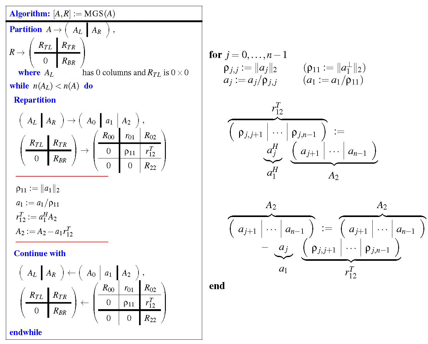
This discussion shows that the updating of future columns by subtracting out the component in the direction of the latest column of \(Q \) to be computed can be cast in terms of a rank-1 update. This is also captured, using FLAME notation, in the algorithm in Figure 3.2.4.2, as is further illustrated in Figure 3.2.4.4:
Ponder This 3.2.4.2.
Let \(A \) have linearly independent columns and let \(A = Q R \) be a QR factorization of \(A \text{.}\) Partition
where \(A_L \) and \(Q_L \) have \(k \) columns and \(R_{TL} \) is \(k \times k \text{.}\)
As you prove the following insights, relate each to the algorithm in Figure 3.2.4.4. In particular, at the top of the loop of a typical iteration, how have the different parts of \(A \) and \(R \) been updated?
-
\(A_L = Q_L R_{TL}\text{.}\)
(\(Q_L R_{TL} \) equals the QR factorization of \(A_L \text{.}\))
-
\({\cal C}( A_L ) = {\cal C}( Q_L ) \text{.}\)
(The first \(k\) columns of \(Q \) form an orthonormal basis for the space spanned by the first \(k \) columns of \(A \text{.}\))
\(R_{TR} = Q_L^H A_R\text{.}\)
-
\((A_R - Q_L R_{TR} )^H Q_L = 0 \text{.}\)
(Each column in \(A_R - Q_L R_{TR}\) equals the component of the corresponding column of \(A_R \) that is orthogonal to \(\Span( Q_L ) \text{.}\))
\({\cal C}( A_R - Q_L R_{TR} ) = {\cal C}( Q_R ) \text{.}\)
-
\(A_R - Q_L R_{TR} = Q_R R_{BR} \text{.}\)
(The columns of \(Q_R \) form an orthonormal basis for the column space of \(A_R - Q_L R_{TR} \text{.}\))
Consider the fact that \(A = Q R \text{.}\) Then, multiplying the partitioned matrices,
Hence
The left equality in (3.2.2) answers 1.
-
\({\cal C}( A_L ) = {\cal C}( Q_L ) \) can be shown by noting that \(R \) is upper triangular and nonsingular and hence \(R_{TL} \) is upper triangular and nonsingular, and using this to show that \({\cal C}( A_L ) \subset {\cal C}( Q_L ) \) and \({\cal C}( Q_L ) \subset {\cal C}( A_L ) \text{:}\)
\({\cal C}( A_L ) \subset {\cal C}( Q_L ) \text{:}\) Let \(y \in {\cal C}( A_L ) \text{.}\) Then there exists \(x \) such that \(A_L x = y \text{.}\) But then \(Q_L R_{TL} x = y \) and hence \(Q_L( R_{TL} x ) = y \) which means that \(y \in {\cal C}( Q_L ) \text{.}\)
\({\cal C}( Q_L ) \subset {\cal C}( A_L ) \text{:}\) Let \(y \in {\cal C}( Q_L ) \text{.}\) Then there exists \(x \) such that \(Q_L x = y \text{.}\) But then \(A_L R_{TL}^{-1} x = y \) and hence \(A_L( R_{TL}^{-1} x ) = y \) which means that \(y \in {\cal C}( A_L ) \text{.}\)
This answers 2.
-
Take \(A_R - Q_L R_{TR} = Q_R R_{BR} \) and multiply both side by \(Q_L^H \text{:}\)
\begin{equation*} Q_L^H( A_R - Q_L R_{TR} )= Q_L^H Q_R R_{BR} \end{equation*}is equivalent to
\begin{equation*} Q_L^H A_R - \begin{array}[t]{c} \underbrace{ Q_L^H Q_L } \\ I \end{array} R_{TR} = \begin{array}[t]{c} \underbrace{ Q_L^H Q_R } \\ 0 \end{array} R_{BR} = 0. \end{equation*}Rearranging yields 3.
-
Since \(A_R - Q_L R_{TR} = Q_R R_{BR} \) we find that \(( A_R - Q_L R_{TR} )^H Q_L = ( Q_R R_{BR} )^H Q_L \) and
\begin{equation*} ( A_R - Q_L R_{TR} )^H Q_L = R_{BR}^H Q_R^H Q_L = 0. \end{equation*} Similar to the proof of 2.
Rearranging the right equality in (3.2.2) yields \(A_R - Q_L R_{TR} = Q_R R_{BR}. \text{,}\) which answers 5.
-
Letting \(\widehat A \) denote the original contents of \(A \text{,}\) at a typical point,
\(A_L \) has been updated with \(Q_L \text{.}\)
\(R_{TL} \) and \(R_{TR} \) have been computed.
\(A_R = \widehat A_R - Q_L R_{TR} \text{.}\)
Homework 3.2.4.3.
Implement the algorithm in Figure 3.2.4.4 as
function [ Aout, Rout ] = MGS_QR( A, R )Input is an \(m \times n \) matrix A and a \(n \times n \) matrix \(R \text{.}\) Output is the matrix \(Q \text{,}\) which has overwritten matrix A, and the upper triangular matrix \(R \text{.}\) (The values below the diagonal can be arbitrary.) You may want to use
Assignments/Week03/matlab/test_MGS_QR.m to check your implementation.