Subsection 2.2.5 Examples of unitary matrices
¶In this unit, we will discuss a few situations where you may have encountered unitary matrices without realizing. Since few of us walk around pointing out to each other "Look, another matrix!", we first consider if a transformation (function) might be a linear transformation. This allows us to then ask the question "What kind of transformations we see around us preserve length?" After that, we discuss how those transformations are represented as matrices. That leaves us to then check whether the resulting matrix is unitary.
Subsubsection 2.2.5.1 Rotations
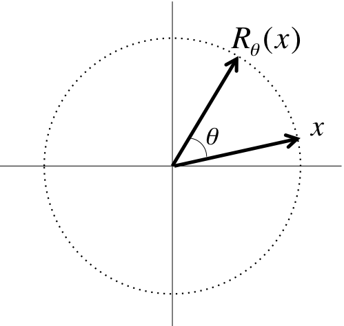
¶A rotation in 2D, \(R_{\theta}: \R^2 \rightarrow \R^2 \text{,}\) takes a vector and rotates that vector through the angle \(\theta \text{:}\)
If you scale a vector first and then rotate it, you get the same result as if you rotate it first and then scale it.
If you add two vectors first and then rotate, you get the same result as if you rotate them first and then add them.
Thus, a rotation is a linear transformation. Also, the above picture captures that a rotation preserves the length of the vector to which it is applied. We conclude that the matrix that represents a rotation should be a unitary matrix.
Let us compute the matrix that represents the rotation through an angle \(\theta \text{.}\) Recall that if \(L : \Cn \rightarrow \Cm \) is a linear transformation and \(A \) is the matrix that represents it, then the \(j \)th column of \(A \text{,}\) \(a_j \text{,}\) equals \(L( e_j ) \text{.}\) The pictures
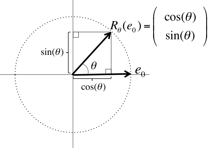
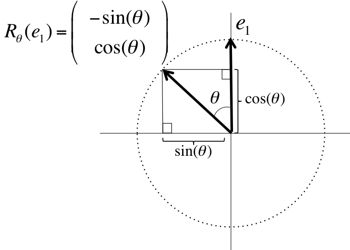
Thus,
Homework 2.2.5.1.
Show that
is a unitary matrix. (Since it is real valued, it is usually called an orthogonal matrix instead.)
Hint: use \(c \) for \(\cos( \theta ) \) and \(s \) for \(\sin( \theta ) \) to save yourself a lot of writing!
Homework 2.2.5.2.
Prove, without relying on geometry but using what you just discovered, that \(\cos( - \theta ) = \cos( \theta ) \) and \(\sin( - \theta ) = - \sin( \theta ) \)
Undoing a rotation by an angle \(\theta \) means rotating in the opposite direction through angle \(\theta \) or, equivalently, rotating through angle \(- \theta \text{.}\) Thus, the inverse of \(R_{\theta} \) is \(R_{-\theta} \text{.}\) The matrix that represents \(R_{\theta} \) is given by
and hence the matrix that represents \(R_{-\theta}\) is given by
Since \(R_{-\theta} \) is the inverse of \(R_{\theta} \) we conclude that
But we just discovered that
Hence
from which we conclude that \(\cos( - \theta ) = \cos( \theta ) \) and \(\sin( - \theta ) = -\sin( \theta ) \text{.}\)
Subsubsection 2.2.5.2 Reflections
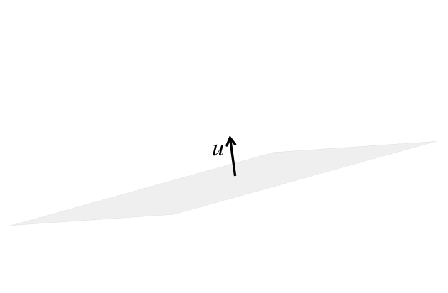
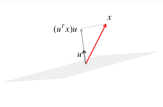
¶Picture a mirror with its orientation defined by a unit length vector, \(u \text{,}\) that is orthogonal to it.
We will consider how a vector, \(x \text{,}\) is reflected by this mirror.

The component of \(x \) orthogonal to the mirror equals the component of \(x \) in the direction of \(u \text{,}\) which equals \((u^T x) u \text{.}\)
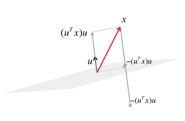
The orthogonal projection of \(x \) onto the mirror is then given by the dashed vector, which equals \(x - (u^Tx) u \text{.}\)

To get to the reflection of \(x \text{,}\) we now need to go further yet by \(-(u^Tx) u \text{.}\)
We conclude that the transformation that mirrors (reflects) \(x \) with respect to the mirror is given by \(M( x ) = x - 2( u^T x ) u \text{.}\)
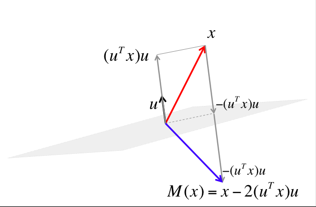
The transformation described above preserves the length of the vector to which it is applied.
Homework 2.2.5.3.
(Verbally) describe why reflecting a vector as described above is a linear transformation.
If you scale a vector first and then reflect it, you get the same result as if you reflect it first and then scale it.
If you add two vectors first and then reflect, you get the same result as if you reflect them first and then add them.
Homework 2.2.5.4.
Show that the matrix that represents \(M: \R^3 \rightarrow \R^3 \) in the above example is given by \(I - 2 u u^T \text{.}\)
Rearrange \(x - 2 ( u^T x ) u \text{.}\)
We notice that
Hence \(M( x ) = ( I -2 u u^T ) x \) and the matrix that represents \(M \) is given by \(I - 2 u u^T \text{.}\)
Homework 2.2.5.5.
(Verbally) describe why \(( I - 2 u u^T )^{-1} = I - 2 u u^T \) if \(u \in \R^3 \) and \(\| u \|_2 = 1 \text{.}\)
If you take a vector, \(x \text{,}\) and reflect it with respect to the mirror defined by \(u \text{,}\) and you then reflect the result with respect to the same mirror, you should get the original vector \(x \) back. Hence, the matrix that represents the reflection should be its own inverse.
Homework 2.2.5.6.
Let \(M: \R^3 \rightarrow \R^3 \) be defined by \(M(x ) = (I - 2 u u^T) x \text{,}\) where \(\| u \|_2 = 1 \text{.}\) Show that the matrix that represents it is unitary (or, rather, orthogonal since it is in \(\R^{3 \times 3} \)).
Pushing through the math we find that
Remark 2.2.5.1.
Unitary matrices in general, and rotations and reflections in particular, will play a key role in many of the practical algorithms we will develop in this course.