Subsection 6.2.4 Stability of a numerical algorithm
¶Correctness in the presence of error (e.g., when floating point computations are performed) takes on a different meaning. For many problems for which computers are used, there is one correct answer and we expect that answer to be computed by our program. The problem is that most real numbers cannot be stored exactly in a computer memory. They are stored as approximations, floating point numbers, instead. Hence storing them and/or computing with them inherently incurs error. The question thus becomes "When is a program correct in the presence of such errors?"
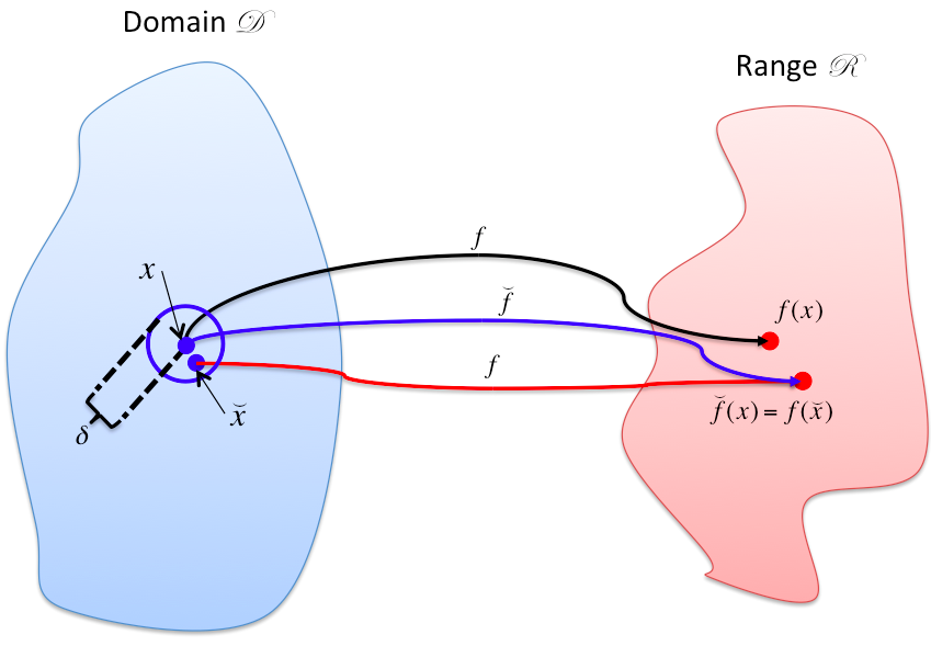
Let us assume that we wish to evaluate the mapping \(f: {\mathcal D} \rightarrow {\mathcal R} \) where \({\mathcal D} \subset \Rn \) is the domain and \({\mathcal R} \subset \Rm \) is the range (codomain). Now, we will let \(\check f: {\mathcal D} \rightarrow {\mathcal R} \) denote a computer implementation of this function. Generally, for \(x \in {\mathcal D} \) it is the case that \(f( x) \neq \check f( x) \text{.}\) Thus, the computed value is not "correct". From earlier discussions about how the condition number of a matrix can amplify relative error, we know that it may not be the case that \(\check f(x) \) is "close to" \(f( x ) \text{:}\) even if \(\check f \) is an exact implementation of \(f \text{,}\) the mere act of storing \(x \) may introduce a small error \(\deltax \) and \(f( x + \deltax ) \) may be far from \(f( x ) \) if \(f \) is ill-conditioned.
The following defines a property that captures correctness in the presence of the kinds of errors that are introduced by computer arithmetic:
Definition 6.2.4.2. Backward stable implementation.
Given the mapping \(f: D \rightarrow R \text{,}\) where \(D \subset \Rn \) is the domain and \(R \subset \Rm \) is the range (codomain), let \(\check f: D \rightarrow R \) be a computer implementation of this function. We will call \(\check f \) a backward stable (also called "numerically stable") implementation of \(f \) on domain \({\mathcal D} \) if for all \(x \in D \) there exists a \(\check x \) "close" to \(x \) such that \(\check f( x ) = f( \check x ) \text{.}\)
The algorithm is said to be forward stable on domain \({\mathcal D} \) if for all \(x \in {\mathcal D} \) it is that case that \(\check f( x ) \approx f( x ) \text{.}\) In other words, the computed result equals a slight perturbation of the exact result.
Example 6.2.4.3.
Under the SCM from the last unit, floating point addition, \(\kappa := \chi + \psi \text{,}\) is a backward stable operation.
where
\(\vert \epsilon_+ \vert \leq \meps \text{,}\)
\(\delta\!\chi = \chi \epsilon_+ \text{,}\)
\(\delta\!\psi = \psi \epsilon_+ \text{.}\)
Hence \(\check \kappa \) equals the exact result when adding nearby inputs.
Homework 6.2.4.1.
ALWAYS/SOMETIMES/NEVER: Under the SCM from the last unit, floating point subtraction, \(\kappa := \chi - \psi \text{,}\) is a backward stable operation.
ALWAYS/SOMETIMES/NEVER: Under the SCM from the last unit, floating point multiplication, \(\kappa := \chi \times \psi \text{,}\) is a backward stable operation.
ALWAYS/SOMETIMES/NEVER: Under the SCM from the last unit, floating point division, \(\kappa := \chi / \psi \text{,}\) is a backward stable operation.
ALWAYS: Under the SCM from the last unit, floating point subtraction, \(\kappa := \chi - \psi \text{,}\) is a backward stable operation.
ALWAYS: Under the SCM from the last unit, floating point multiplication, \(\kappa := \chi \times \psi \text{,}\) is a backward stable operation.
ALWAYS: Under the SCM from the last unit, floating point division, \(\kappa := \chi / \psi \text{,}\) is a backward stable operation.
Now prove it!
-
ALWAYS: Under the SCM from the last unit, floating point subtraction, \(\kappa := \chi - \psi \text{,}\) is a backward stable operation.
\begin{equation*} \begin{array}{l} \check \kappa \\ ~~~ = ~~~~ \lt \mbox{ computed value for } \kappa \gt \\ \left[ \chi - \psi \right] \\ ~~~ = ~~~~ \lt \mbox{ SCM } \gt \\ ( \chi - \psi )( 1 + \epsilon_- ) \\ ~~~ = ~~~~ \lt \mbox{ distribute } \gt \\ \chi ( 1 + \epsilon_- ) - \psi ( 1 + \epsilon_- ) \\ ~~~ = ~~~~ \\ ( \chi +\delta\!\chi ) - ( \psi + \delta\!\psi ) \end{array} \end{equation*}where
\(\vert \epsilon_- \vert \leq \meps \text{,}\)
\(\delta\!\chi = \chi \epsilon_- \text{,}\)
\(\delta\!\psi = \psi \epsilon_- \text{.}\)
Hence \(\check \kappa \) equals the exact result when subtracting nearby inputs.
-
ALWAYS: Under the SCM from the last unit, floating point multiplication, \(\kappa := \chi \times \psi \text{,}\) is a backward stable operation.
\begin{equation*} \begin{array}{l} \check \kappa \\ ~~~ = ~~~~ \lt \mbox{ computed value for } \kappa \gt \\ \left[ \chi \times \psi \right] \\ ~~~ = ~~~~ \lt \mbox{ SCM } \gt \\ ( \chi \times \psi )( 1 + \epsilon_\times ) \\ ~~~ = ~~~~ \lt \mbox{ associative property } \gt \\ \chi \times \psi ( 1 + \epsilon_\times ) \\ ~~~ = ~~~~ \\ \chi ( \psi + \delta\!\psi ) \end{array} \end{equation*}where
\(\vert \epsilon_\times \vert \leq \meps \text{,}\)
\(\delta\!\psi = \psi \epsilon_\times \text{.}\)
Hence \(\check \kappa \) equals the exact result when multiplying nearby inputs.
-
ALWAYS: Under the SCM from the last unit, floating point division, \(\kappa := \chi / \psi \text{,}\) is a backward stable operation.
\begin{equation*} \begin{array}{l} \check \kappa \\ ~~~ = ~~~~ \lt \mbox{ computed value for } \kappa \gt \\ \left[ \chi / \psi \right] \lt \\ ~~~ = ~~~~ \mbox{ SCM } \gt \\ ( \chi / \psi )( 1 + \epsilon_/ ) \\ ~~~ = ~~~~ \lt \mbox{ commutative property } \gt \\ \chi ( 1 + \epsilon_/ ) / \psi \\ ~~~ = ~~~~ \\ ( \chi +\delta\!\chi ) / \psi \end{array} \end{equation*}where
\(\vert \epsilon_/ \vert \leq \meps \text{,}\)
\(\delta\!\chi = \chi \epsilon_/ \text{,}\)
Hence \(\check \kappa \) equals the exact result when dividing nearby inputs.
Ponder This 6.2.4.2.
In the last homework, we showed that floating point division is backward stable by showing that \(\left[ \chi / \psi \right] = (\chi + \delta\!\chi) / \psi \) for suitably small \(\delta\!\chi \text{.}\)
How would one show that \(\left[ \chi / \psi \right] = \chi / ( \psi + \delta\!\psi ) \) for suitably small \(\delta\!\psi \text{?}\)