Subsection 7.2.2 Nested dissection
¶The purpose of the game is to limit fill-in, which happens when zeroes turn into nonzeroes. With an example that would result from, for example, Poisson's equation, we will illustrate the basic techniques, which are known as "nested dissection."
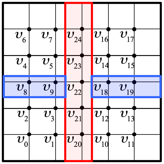
If you consider the mesh that results from the discretization of, for example, a square domain, the numbering of the mesh points does not need to be according to the "natural ordering" we chose to use before. As we number the mesh points, we reorder (permute) both the columns of the matrix (which correspond to the elements \(\upsilon_i \) to be computed) and the equations that tell one how \(\upsilon_i \) is computed from its neighbors. If we choose a separator, the points highlighted in red in Figure 7.2.2.1 (Top-Left), and order the mesh points to its left first, then the ones to its right, and finally the points in the separator, we create a pattern of zeroes, as illustrated in Figure 7.2.2.1 (Top-Right).

Homework 7.2.2.1.
Consider the SPD matrix
What special structure does the Cholesky factor of this matrix have?
How can the different parts of the Cholesky factor be computed in a way that takes advantage of the zero blocks?
How do you take advantage of the zero pattern when solving with the Cholesky factors?
-
The Cholesky factor of this matrix has the structure
\begin{equation*} L = \left( \begin{array}{c | c | c} L_{00} \amp 0 \amp 0\\ \hline 0 \amp L_{11} \amp 0 \\ \hline L_{20} \amp L_{21} \amp L_{22} \end{array} \right). \end{equation*} -
We notice that \(A = L L^T \) means that
\begin{equation*} \left( \begin{array}{c | c | c} A_{00} \amp 0 \amp A_{20}^T \\ \hline 0 \amp A_{11} \amp A_{21}^T \\ \hline A_{20} \amp A_{21} \amp A_{22} \end{array} \right) = \begin{array}[t]{c} \underbrace{ \left( \begin{array}{c | c | c} L_{00} \amp 0 \amp 0\\ \hline 0 \amp L_{11} \amp 0 \\ \hline L_{20} \amp L_{21} \amp L_{22} \end{array} \right) \left( \begin{array}{c | c | c} L_{00} \amp 0 \amp 0\\ \hline 0 \amp L_{11} \amp 0 \\ \hline L_{20} \amp L_{21} \amp L_{22} \end{array} \right)^T, } \\ \left( \begin{array}{c | c | c} L_{00} L_{00}^T\amp 0 \amp \star\\ \hline 0 \amp L_{11} L_{11}^T \amp \star \\ \hline L_{20} L_{00}^T \amp L_{21} L_{11}^T \amp L_{20} L_{20}^T + L_{21} L_{21}^T + L_{22} L_{22}^T \end{array} \right) \end{array} \end{equation*}where the \(\star\)s indicate "symmetric parts" that don't play a role. We deduce that the following steps will yield the Cholesky factor:
-
Compute the Cholesky factor of \(A_{00} \text{:}\)
\begin{equation*} A_{00} = L_{00} L_{00}^T, \end{equation*}overwriting \(A_{00} \) with the result.
-
Compute the Cholesky factor of \(A_{11} \text{:}\)
\begin{equation*} A_{11} = L_{11} L_{11}^T, \end{equation*}overwriting \(A_{11} \) with the result.
-
Solve
\begin{equation*} X L_{00}^T = A_{20} \end{equation*}for \(X \text{,}\) overwriting \(A_{20} \) with the result. (This is a triangular solve with multiple right-hand sides in disguise.)
-
Solve
\begin{equation*} X L_{11}^T = A_{21} \end{equation*}for \(X \text{,}\) overwriting \(A_{21} \) with the result. (This is a triangular solve with multiple right-hand sides in disguise.)
-
Update the lower triangular part of \(A_{22}\) with
\begin{equation*} A_{22} - L_{20} L_{20}^T - L_{21} L_{21}^T. \end{equation*} -
Compute the Cholesky factor of \(A_{22} \text{:}\)
\begin{equation*} A_{22} = L_{22} L_{22}^T, \end{equation*}overwriting \(A_{22} \) with the result.
-
-
If we now want to solve \(A x = y \text{,}\) we can instead first solve \(L z = y \) and then \(L^T x = z \text{.}\) Consider
\begin{equation*} \left( \begin{array}{c | c | c} L_{00} \amp 0 \amp 0\\ \hline 0 \amp L_{11} \amp 0 \\ \hline L_{20} \amp L_{21} \amp L_{22} \end{array} \right) \left( \begin{array}{c} z_0 \\ \hline z_1 \\ \hline z_2 \end{array} \right) = \left( \begin{array}{c} y_0 \\ \hline y_1 \\ \hline y_2 \end{array} \right) . \end{equation*}This can be solved via the steps
Solve \(L_{00} z_0 = y_0 \text{.}\)
Solve \(L_{11} z_1 = y_1 \text{.}\)
Solve \(L_{22} z_2 = y_2 - L_{20} z_0 - L_{21} z_1 \text{.}\)
Similarly,
\begin{equation*} \left( \begin{array}{c | c | c} L_{00}^T \amp 0 \amp L_{20}^T\\ \hline 0 \amp L_{11}^T \amp L_{21}^T \\ \hline 0 \amp 0 \amp L_{22}^T \end{array} \right) \left( \begin{array}{c} x_0 \\ \hline x_1 \\ \hline x_2 \end{array} \right) = \left( \begin{array}{c} z_0 \\ \hline z_1 \\ \hline z_2 \end{array} \right) . \end{equation*}can be solved via the steps
Solve \(L_{22}^T x_2 = z_2 \text{.}\)
Solve \(L_{11}^T x_1 = z_1 - L_{21}^T x_2 \text{.}\)
Solve \(L_{00}^T x_0 = z_0 - L_{20}^T x_2 \text{.}\)
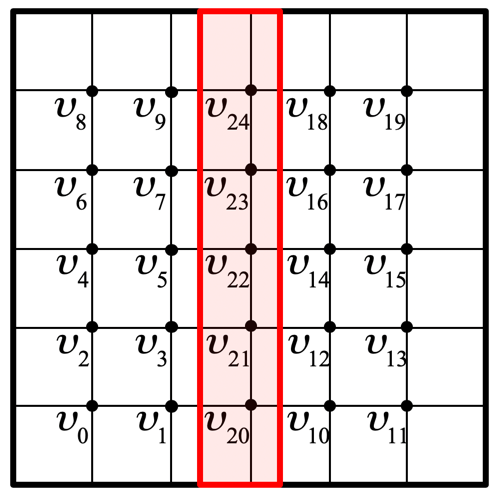
Each of the three subdomains that were created in Figure 7.2.2.1 can themselves be reordered by identifying separators. In Figure 7.2.2.2 we illustrate this only for the left and right subdomains. This creates a recursive structure in the matrix. Hence, the name nested dissection for this approach.