Subsection 12.1.1 Simple Implementation of matrix-matrix multiplication
¶The current coronavirus crisis hit UT-Austin on March 14, 2020, a day we spent quickly making videos for Week 11. We have not been back to the office, to create videos for Week 12, since then. We will likely add such videos as time goes on. For now, we hope that the notes suffice.
Remark 12.1.1.1.
The exercises in this unit assume that you have installed the BLAS-like Library Instantiation Software (BLIS), as described in Subsection 0.2.4.
Let \(A \text{,}\) \(B \text{,}\) and \(C \) be \(m \times k \text{,}\) \(k \times n \text{,}\) and \(m \times n \) matrices, respectively. We can expose their individual entries as
and
The computation \(C := A B + C \text{,}\) which adds the result of the matrix-matrix multiplication \(A B \) to a matrix \(C \text{,}\) is defined element-wise as
for all \(0 \leq i \lt m \) and \(0 \leq j \lt n \text{.}\) We add to \(C \) because this will make it easier to play with the orderings of the loops when implementing matrix-matrix multiplication. The following pseudo-code computes \(C := A B + C \text{:}\)
The outer two loops visit each element of \(C \) and the inner loop updates \(\gamma_{i,j} \) with (12.1.1). We use C programming language macro definitions in order to explicitly index into the matrices, which are passed as one-dimentional arrays in which the matrices are stored in column-major order.
Remark 12.1.1.2.
For a more complete discussion of how matrices are mapped to memory, you may want to look at 1.2.1 Mapping matrices to memory in our MOOC titled LAFF-On Programming for High Performance. If the discussion here is a bit too fast, you may want to consult the entire Section 1.2 Loop orderings of that course.
#define alpha( i,j ) A[ (j)*ldA + i ]   // map alpha( i,j ) to array A
#define beta( i,j )  B[ (j)*ldB + i ]   // map beta( i,j )  to array B
#define gamma( i,j ) C[ (j)*ldC + i ]   // map gamma( i,j ) to array C

void MyGemm( int m, int n, int k, double *A, int ldA,
	     double *B, int ldB, double *C, int ldC )
{
  for ( int i=0; i<m; i++ )
    for ( int j=0; j<n; j++ )
      for ( int p=0; p<k; p++ )
        gamma( i,j ) += alpha( i,p ) * beta( p,j );
}
Homework 12.1.1.1.
In the file Assignments/Week12/C/Gemm_IJP.c you will find the simple implementation given in Figure 12.1.1.3 that computes \(C := A B + C
\text{.}\) In a terminal window, the directory Assignments/Week12/C, execute
make IJPto compile, link, and execute it. You can view the performance attained on your computer with the Matlab Live Script in
Assignments/Week12/C/data/Plot_IJP.mlx (Alternatively, read and execute Assignments/Week12/C/data/Plot_IJP_m.m.)On Robert's laptop, Homework 12.1.1.1 yields the graph
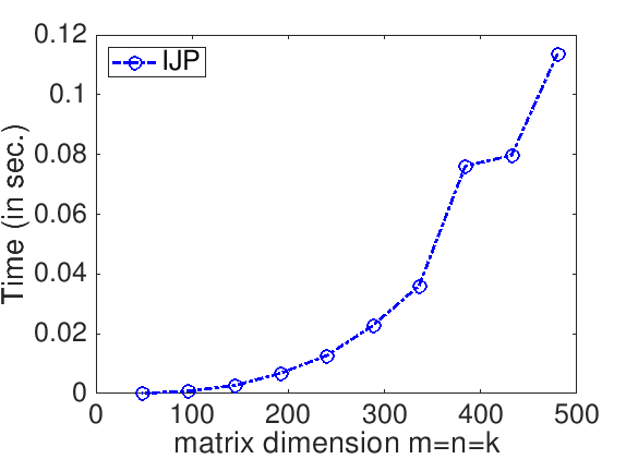
IJP. The time, in seconds, required to compute matrix-matrix multiplication as a function of the matrix size is plotted, where \(m = n = k \) (each matrix is square). "Irregularities" in the time required to complete can be attributed to a number of factors, including that other processes that are executing on the same processor may be disrupting the computation. One should not be too concerned about those.
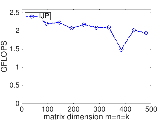
The performance of a matrix-matrix multiplication implementation is measured in billions of floating point operations per second (GFLOPS). We know that it takes \(2 m n k \) flops to compute \(C := A B + C \) when \(C \) is \(m \times n \text{,}\) \(A\) is \(m \times k \text{,}\) and \(B \) is \(k \times n \text{.}\) If we measure the time it takes to complete the computation, \(T( m, n, k ) \text{,}\) then the rate at which we compute is given by
For our implementation, this yields
Remark 12.1.1.4.
The Gemm in the name of the routine stands for General Matrix-Matrix multiplication. Gemm is an acronym that is widely used in scientific computing, with roots in the Basic Linear Algebra Subprograms (BLAS) interface which we will discuss in Subsection 12.2.5.
Homework 12.1.1.2.
The IJP ordering is one possible ordering of the loops. How many distinct reorderings of those loops are there?
There are three choices for the outer-most loop: \(i \text{,}\) \(j \text{,}\) or \(p \text{.}\)
Once a choice is made for the outer-most loop, there are two choices left for the second loop.
Once that choice is made, there is only one choice left for the inner-most loop.
Thus, there are \(3! = 3 \times 2 \times 1 = 6 \) loop orderings.
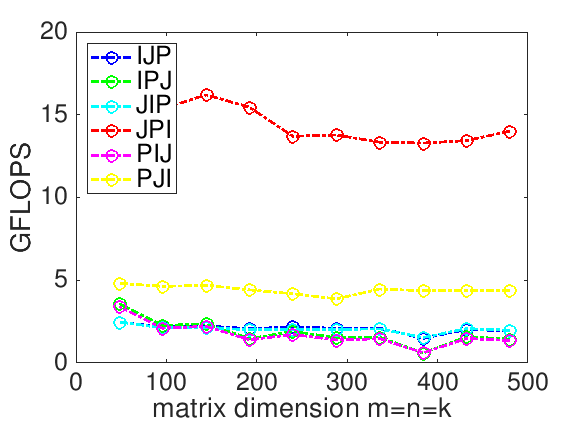
Homework 12.1.1.3.
In directory Assignments/Week12/C make copies of Assignments/Week12/C/Gemm_IJP.c into files with names that reflect the different loop orderings (Gemm_IPJ.c, etc.). Next, make the necessary changes to the loops in each file to reflect the ordering encoded in its name. Test the implementions by executing
make IPJ
make JIP
   ...
for each of the implementations and view the resulting performance by making the indicated changes to the Live Script in
Assignments/Week12/C/data/Plot_All_Orderings.mlx (Alternatively, use the script in Assignments/Week12/C/data/Plot_All_Orderings_m.m). If you have implemented them all, you can test them all by executing make All_Orderings
Homework 12.1.1.4.
In directory Assignments/Week12/C/ execute
make JPIand view the results with the Live Script in
Assignments/Week12/C/data/Plot_Opener.mlx. (This may take a little while, since the Makefile now specifies that the largest problem to be executed is \(m=n=k=1500\text{.}\))
Next, change that Live Script to also show the performance of the reference implementation provided by the BLAS-like Library Instantion Software (BLIS): Change
% Optionally show the reference implementation performance data
if ( 0 )
to
% Optionally show the reference implementation performance data
if ( 1 )
and rerun the Live Script. This adds a plot to the graph for the reference implementation.
What do you observe? Now are you happy with the improvements you made by reordering the loops>
On Robert's laptop:
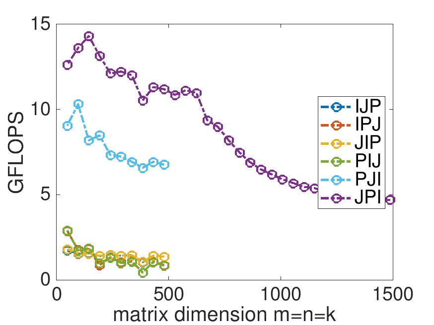
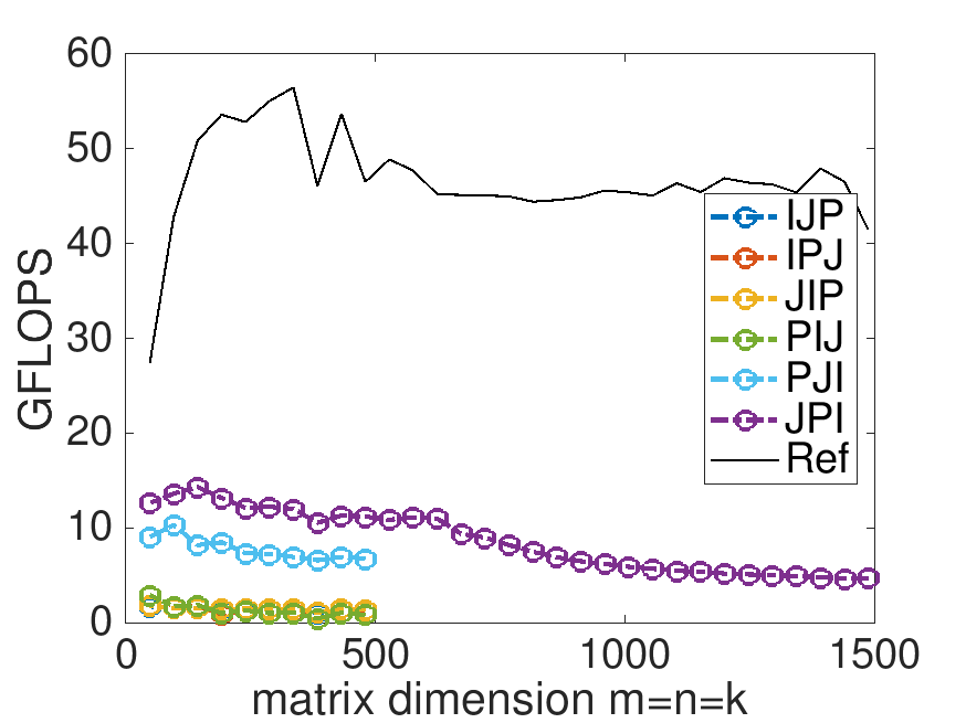
Note: the performance in the graph on the left may not exactly match that in the graph earlier in this unit. My laptop does not always attain the same performance. When a processor gets hot, it "clocks down." This means the attainable performance goes down. A laptop is not easy to cool, so one would expect more fluctuation than when using, for example, a desktop or a server.
Here is a video from our course "LAFF-On Programming for High Performance", which explains what you observe. (It refers to "Week 1" or that course. It is part of the launch for that course.)
Remark 12.1.1.6.
There are a number of things to take away from the exercises in this unit.
The ordering of the loops matters. Why? Because it changes the pattern of memory access. Accessing memory contiguously (what is often called "with stride one") improves performance.
Compilers, which translate high-level code written in a language like C, are not the answer. You would think that they would reorder the loops to improve performance. The widely-used
gcccompiler doesn't do so very effectively. (Intel's highly-acclaimedicccompiler does a much better job, but still does not produce performance that rivals the reference implementation.)Careful implementation can greatly improve performance.
One solution is to learn how to optimize yourself. Some of the fundamentals can be discovered in our MOOC LAFF-On Programming for High Performance. The other solution is to use highly optimized libraries, some of which we will discuss later in this week.