Unit 1.1.1 Launch
¶Homework 1.1.1.1.
Compute \(\left(\begin{array}{rrr} 1 \amp -2 \amp 2\\ 1 \amp 1 \amp 3\\ -2 \amp 2 \amp 1 \end{array}\right) \left(\begin{array}{rr} -2 \amp 1\\ 1 \amp 3\\ -1 \amp 2 \end{array}\right) + \left(\begin{array}{rr} 1 \amp 0\\ -1 \amp 2\\ -2 \amp 1 \end{array}\right) = \)
\(\left(\begin{array}{rrr} 1 \amp -2 \amp 2\\ 1 \amp 1 \amp 3\\ -2 \amp 2 \amp 1 \end{array}\right) \left(\begin{array}{rr} -2 \amp 1\\ 1 \amp 3\\ -1 \amp 2 \end{array}\right) + \left(\begin{array}{rr} 1 \amp 0\\ -1 \amp 2\\ -2 \amp 1 \end{array}\right) = \left(\begin{array}{rr} -5 \amp -1\\ -5 \amp 12\\ 3 \amp 7 \end{array}\right)\)
Let us explicitly define some notation that we will use to discuss matrix-matrix multiplication more abstractly.
Let \(A \text{,}\) \(B \text{,}\) and \(C \) be \(m \times k \text{,}\) \(k \times n \text{,}\) and \(m \times n \) matrices, respectively. We can expose their individual entries as
and
The computation \(C := A B + C \text{,}\) which adds the result of matrix-matrix multiplication \(A B \) to a matrix \(C \text{,}\) is defined as
for all \(0 \leq i \lt m \) and \(0 \leq j \lt n \text{.}\) Why we add to \(C \) will become clear later. This leads to the following pseudo-code for computing \(C := A B + C \text{:}\)
The outer two loops visit each element of \(C \text{,}\) and the inner loop updates \(\gamma_{i,j} \) with (1.1.1).
#define alpha( i,j ) A[ (j)*ldA + i ]   // map alpha( i,j ) to array A
#define beta( i,j )  B[ (j)*ldB + i ]   // map beta( i,j )  to array B
#define gamma( i,j ) C[ (j)*ldC + i ]   // map gamma( i,j ) to array C

void MyGemm( int m, int n, int k, double *A, int ldA,
	     double *B, int ldB, double *C, int ldC )
{
  for ( int i=0; i<m; i++ )
    for ( int j=0; j<n; j++ )
      for ( int p=0; p<k; p++ )
        gamma( i,j ) += alpha( i,p ) * beta( p,j );
}
Homework 1.1.1.2.
In the file Assignments/Week1/C/Gemm_IJP.c you will find the simple implementation given in Figure 1.1.1 that computes \(C := A B + C
\text{.}\) In the directory Assignments/Week1/C execute
make IJPto compile, link, and execute it. You can view the performance attained on your computer with the Matlab Live Script in
Assignments/Week1/C/data/Plot_IJP.mlx (Alternatively, read and execute Assignments/Week1/C/data/Plot_IJP_m.m.)On Robert's laptop, Homework 1.1.1.2 yields the graph
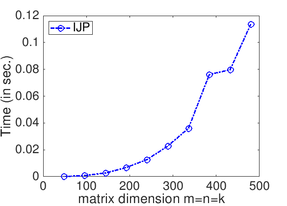
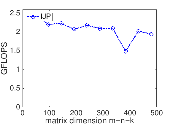
The performance of a matrix-matrix multiplication implementation is measured in billions of floating point operations (flops) per second (GFLOPS). The idea is that we know that it takes \(2 m n k \) flops to compute \(C := A B + C \) where \(C \) is \(m \times n \text{,}\) \(A\) is \(m \times k \text{,}\) and \(B \) is \(k \times n \text{.}\) If we measure the time it takes to complete the computation, \(T( m, n, k ) \text{,}\) then the rate at which we compute is given by
For our implementation and the reference implementation, this yields
Remark 1.1.2.
The Gemm in the name of the routine stands for General Matrix-Matrix multiplication. Gemm is an acronym that is widely used in scientific computing, with roots in the Basic Linear Algebra Subprograms (BLAS) discussed in the enrichment in Unit 1.5.1.