Unit 1.4.4 Matrix-matrix multiplication via row-times-matrix multiplications
¶Finally, let us partition \(C \) and \(A \) by rows so that
\begin{equation*}
\begin{array}{rcl}
\left( \begin{array}{c}
\widetilde c_0^T \\ \hline
\widetilde c_1^T \\ \hline
\vdots \\ \hline
\widetilde c_{m-1}^T
\end{array} \right) \amp:=\amp
\left( \begin{array}{c}
\widetilde a_0^T \\ \hline
\widetilde a_1^T \\ \hline
\vdots \\ \hline
\widetilde a_{m-1}^T
\end{array} \right) B
+
\left( \begin{array}{c}
\widetilde c_0^T \\ \hline
\widetilde c_1^T \\ \hline
\vdots \\ \hline
\widetilde c_{m-1}^T
\end{array} \right)
=
\left( \begin{array}{c}
\widetilde a_0^T B + \widetilde c_0^T \\ \hline
\widetilde a_1^T B + \widetilde c_1^T \\ \hline
\vdots \\ \hline
\widetilde a_{m-1}^T B + \widetilde c_{m-1}^T
\end{array} \right)
\end{array}
\end{equation*}
A picture that captures this is given by
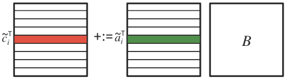
This illustrates how the IJP and IPJ algorithms can be viewed as a loop around the updating of a row of \(C \) with the product of the corresponding row of \(A \) times matrix \(B \text{:}\)
\begin{equation*}
\begin{array}{l}
{\bf for~} i := 0, \ldots , m-1 \\[0.15in]
~~~
\left. \begin{array}{l}
{\bf for~} j := 0, \ldots , n-1 \\[0.15in]
~~~ ~~~
\left. \begin{array}{l}
{\bf for~} p := 0, \ldots , k-1 \\
~~~ ~~~ \gamma_{i,j} := \alpha_{i,p} \beta_{p,j} + \gamma_{i,j} \\
{\bf end}
\end{array} \right\} ~~~ \begin{array}[t]{c}
\underbrace{\widetilde \gamma_{i,j} := \widetilde a_i^T b_j +
\widetilde \gamma_{i,j}}\\
\mbox{dot}
\end{array}
\\[0.2in]
~~~ {\bf end}
\end{array} \right\} ~~~ \begin{array}[t]{c}
\underbrace{
\widetilde c_i^T := \widetilde a_i^T B + \widetilde c_i^T}
\\
\mbox{row-matrix mult}
\end{array}
\\[0.2in]
{\bf end}
\end{array}
\end{equation*}
and
\begin{equation*}
\begin{array}{l}
{\bf for~} i := 0, \ldots , m-1 \\[0.15in]
~~~
\left. \begin{array}{l}
{\bf for~} p := 0, \ldots , k-1 \\[0.15in]
~~~ ~~~
\left. \begin{array}{l}
{\bf for~} j := 0, \ldots , n-1 \\
~~~ ~~~ \gamma_{i,j} := \alpha_{i,p} \beta_{p,j} + \gamma_{i,j} \\
{\bf end}
\end{array} \right\} ~~~ \begin{array}[t]{c}
\underbrace{\widetilde c_i^T :=
\alpha_{i,p} \widetilde b_p^T + \widetilde c_i^T}\\
\mbox{axpy}
\end{array}
\\[0.2in]
~~~ {\bf end}
\end{array} \right\} ~~~ \begin{array}[t]{c}
\underbrace{\widetilde c_i^T := \widetilde a_i^T B + \widetilde
c_i^T}\\
\mbox{row-matrix mult}
\end{array}
\\[0.2in]
{\bf end}
\end{array}
\end{equation*}
The problem with implementing the above algorithms is that Gemv_I_Dots and Gemv_J_Axpy implement \(y := A x + y \) rather than \(y^T := x^T A + y^T \text{.}\) Obviously, you could create new routines for this new operation. We will get back to this in the "Additional Exercises" section of this chapter.