Unit 1.6.2 Summary
¶The building blocks for matrix-matrix multiplication (and many matrix algorithms) are
-
Vector-vector operations:
Dot: \(x^T y \text{.}\)
Axpy: \(y := \alpha x + y \text{.}\)
-
Matrix-vector operations:
Matrix-vector multiplication: \(y := A x + y\) and \(y := A^T x + y \text{.}\)
Rank-1 update: \(A := x y^T + A \text{.}\)
Partitioning the matrices by rows and colums, with these operations, the matrix-matrix multiplication \(C := A B + C \) can be described as one loop around
-
multiple matrix-vector multiplications:
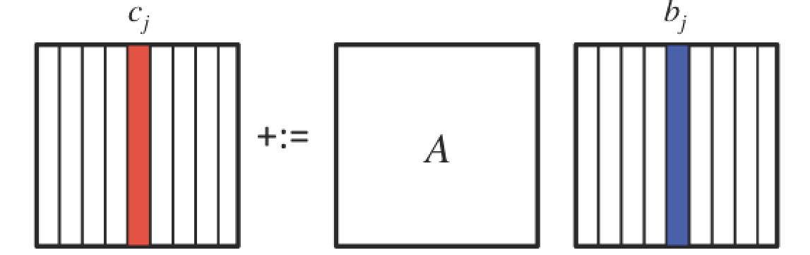
\begin{equation*} \left( \begin{array}{c | c | c } c_0 \amp \cdots \amp c_{n-1} \end{array} \right) := \left( \begin{array}{c | c | c } A b_0 + c_0 \amp \cdots \amp A b_{n-1} + c_{n-1} \end{array} \right) \end{equation*}illustrated by
.
This hides the two inner loops of the triple nested loop in the matrix-vector multiplication:
\begin{equation*} \begin{array}{l} {\bf for~} j := 0, \ldots , n-1 \\[0.15in] ~~~ \left. \begin{array}{l} {\bf for~} p := 0, \ldots , k-1 \\[0.15in] ~~~ ~~~ \left. \begin{array}{l} {\bf for~} i := 0, \ldots , m-1 \\ ~~~ ~~~ \gamma_{i,j} := \alpha_{i,p} \beta_{p,j} + \gamma_{i,j} \\ {\bf end} \end{array} \right\} ~~~ \begin{array}[t]{c} \underbrace{c_j := \beta_{p,j} a_p + c_j}\\ \mbox{axpy} \end{array} \\[0.2in] ~~~ {\bf end} \end{array} \right\} ~~~ \begin{array}[t]{c} \underbrace{c_j := A b_j + c_j}\\ \mbox{mv mult} \end{array} \\[0.2in] {\bf end} \end{array} \end{equation*}and
\begin{equation*} \begin{array}{l} {\bf for~} j := 0, \ldots , n-1 \\[0.15in] ~~~ \left. \begin{array}{l} {\bf for~} i := 0, \ldots , m-1 \\[0.15in] ~~~ ~~~ \left. \begin{array}{l} {\bf for~} p := 0, \ldots , k-1 \\ ~~~ ~~~ \gamma_{i,j} := \begin{array}[t]{c} \underbrace{\alpha_{i,p} \beta_{p,j} + \gamma_{i,j}}\\ \mbox{axpy} \end{array} \\ {\bf end} \end{array} \right\} ~~~ \gamma_{i,j} := \widetilde a_i^T b_j + \gamma_{i,j} \\[0.2in] ~~~ {\bf end} \end{array} \right\} ~~~ \begin{array}[t]{c} \underbrace{c_j := A b_j + c_j}\\ \mbox{mv mult} \end{array} \\[0.2in] {\bf end} \end{array} \end{equation*} -
multiple rank-1 updates:
\begin{equation*} C := a_0 \widetilde b_0^T + a_1 \widetilde b_1^T + \cdots + a_{k-1} \widetilde b_{k-1}^T + C \end{equation*}illustrated by
This hides the two inner loops of the triple nested loop in the rank-1 update: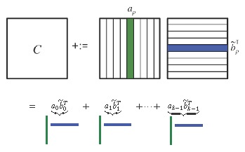 \begin{equation*} \begin{array}{l} {\bf for~} p := 0, \ldots , k-1 \\[0.15in] ~~~ \left. \begin{array}{l} {\bf for~} j := 0, \ldots , n-1 \\[0.15in] ~~~ ~~~ \left. \begin{array}{l} {\bf for~} i := 0, \ldots , m-1 \\ ~~~ ~~~ \gamma_{i,j} := \alpha_{i,p} \beta_{p,j} + \gamma_{i,j} \\ {\bf end} \end{array} \right\} ~~~ \begin{array}[t]{c} \underbrace{c_j := \beta_{p,j} a_p + c_j}\\ \mbox{axpy} \end{array} \\[0.2in] ~~~ {\bf end} \end{array} \right\} ~~~ \begin{array}[t]{c} \underbrace{C := a_p \widetilde b_p^T + C}\\ \mbox{rank-1 update} \end{array} \\[0.2in] {\bf end} \end{array} \end{equation*}
and
\begin{equation*} \begin{array}{l} {\bf for~} p := 0, \ldots , k-1 \\[0.15in] ~~~ \left. \begin{array}{l} {\bf for~} i := 0, \ldots , m-1 \\[0.15in] ~~~ ~~~ \left. \begin{array}{l} {\bf for~} j := 0, \ldots , n-1 \\ ~~~ ~~~ \gamma_{i,j} := \alpha_{i,p} \beta_{p,j} + \gamma_{i,j} \\ {\bf end} \end{array} \right\} ~~~ \begin{array}[t]{c} \underbrace{\widetilde c_i^T := \alpha_{i,p} \widetilde b_p^T + \widetilde c_i^T}\\ \mbox{axpy} \end{array} \\[0.2in] ~~~ {\bf end} \end{array} \right\} ~~~ \begin{array}[t]{c} \underbrace{C := a_p \widetilde b_p^T + C}\\ \mbox{rank-1 update} \end{array} \\[0.2in] {\bf end} \end{array} \end{equation*} -
multiple row times matrix multiplications:
\begin{equation*} \left( \begin{array}{c} \widetilde c_0^T \\ \hline \widetilde c_1^T \\ \hline \vdots \\ \hline \widetilde c_{m-1}^T \end{array} \right) := \left( \begin{array}{c} \widetilde a_0^T B + \widetilde c_0^T \\ \hline \widetilde a_1^T B + \widetilde c_1^T \\ \hline \vdots \\ \hline \widetilde a_{m-1}^T B + \widetilde c_{m-1}^T \end{array} \right) \end{equation*}illustrated by
This hides the two inner loops of the triple nested loop in multiplications of rows with matrix \(B \text{:}\)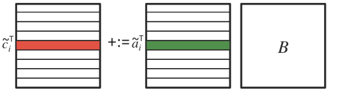 \begin{equation*} \begin{array}{l} {\bf for~} i := 0, \ldots , m-1 \\[0.15in] ~~~ \left. \begin{array}{l} {\bf for~} j := 0, \ldots , n-1 \\[0.15in] ~~~ ~~~ \left. \begin{array}{l} {\bf for~} p := 0, \ldots , k-1 \\ ~~~ ~~~ \gamma_{i,j} := \alpha_{i,p} \beta_{p,j} + \gamma_{i,j} \\ {\bf end} \end{array} \right\} ~~~ \begin{array}[t]{c} \underbrace{\widetilde \gamma_{i,j} := \widetilde a_i^T b_j + \widetilde \gamma_{i,j}}\\ \mbox{dot} \end{array} \\[0.2in] ~~~ {\bf end} \end{array} \right\} ~~~ \begin{array}[t]{c} \underbrace{ \widetilde c_i^T := \widetilde a_i^T B + \widetilde c_i^T} \\ \mbox{row-matrix mult} \end{array} \\[0.2in] {\bf end} \end{array} \end{equation*}
and
\begin{equation*} \begin{array}{l} {\bf for~} i := 0, \ldots , m-1 \\[0.15in] ~~~ \left. \begin{array}{l} {\bf for~} p := 0, \ldots , k-1 \\[0.15in] ~~~ ~~~ \left. \begin{array}{l} {\bf for~} j := 0, \ldots , n-1 \\ ~~~ ~~~ \gamma_{i,j} := \alpha_{i,p} \beta_{p,j} + \gamma_{i,j} \\ {\bf end} \end{array} \right\} ~~~ \begin{array}[t]{c} \underbrace{\widetilde c_i^T := \alpha_{i,p} \widetilde b_p^T + \widetilde c_i^T}\\ \mbox{axpy} \end{array} \\[0.2in] ~~~ {\bf end} \end{array} \right\} ~~~ \begin{array}[t]{c} \underbrace{\widetilde c_i^T := \widetilde a_i^T B + \widetilde c_i^T}\\ \mbox{row-matrix mult} \end{array} \\[0.2in] {\bf end} \end{array} \end{equation*}
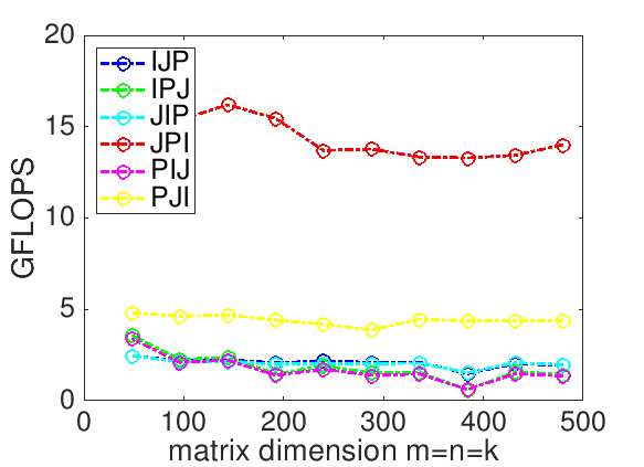
This summarizes all six loop orderings for matrix-matrix multiplication.
While it would be tempting to hope that a compiler would translate any of the six loop orderings into high-performance code, this is an optimistic dream. Our experiments shows that the order in which the loops are ordered has a nontrivial effect on performance:
Those who did the additional exercises in Unit 1.6.1 found out that casting compution in terms of matrix-vector or rank-1 update operations in the BLIS typed API or the BLAS interface, when linked to an optimized implementation of those interfaces, yields better performance.