Unit 2.3.5 Alternative view
¶We can arrive at the same algorithm by partitioning
\begin{equation*}
C = \left( \begin{array}{c | c | c | c }
C_{0,0} \amp C_{0,1} \amp \cdots \amp C_{0,N-1} \\ \hline
C_{1,0} \amp C_{1,1} \amp \cdots \amp C_{1,N-1} \\ \hline
\vdots \amp \vdots \amp \amp \vdots \\ \hline
C_{M-1,0} \amp C_{M,1} \amp \cdots \amp C_{M-1,N-1}
\end{array} \right),
A = \left( \begin{array}{c }
A_{0} \\ \hline
A_{1} \\ \hline
\vdots \\ \hline
A_{M-1}
\end{array} \right),
\end{equation*}
and
\begin{equation*}
B = \left( \begin{array}{c | c | c | c }
B_{0} \amp B_{1} \amp \cdots \amp B_{0,N-1}
\end{array} \right),
\end{equation*}
where \(C_{i,j} \) is \(m_R \times n_R \text{,}\) \(A_i \) is \(m_R \times k \text{,}\) and \(B_j \) is \(k \times n_R \text{.}\) Then computing \(C := A B + C \) means updating \(C_{i,j} := A_i B_j + C_{i,j} \) for all \(i, j \text{:}\)
\begin{equation*}
\begin{array}{l}
\begin{array}{l}
{\bf for~} j := 0, \ldots , N-1 \\[0.05in]
~~~
\left. \begin{array}{l}
{\bf for~} i := 0, \ldots , M-1 \\[0.05in]
~~~ ~~~
\left. \begin{array}{l}
C_{i,j} := A_i B_j + C_{i,j}
\end{array} \right. ~~~ \mbox{Computed with the micro-kernel} \\[0.1in]
~~~ {\bf end}
\end{array}\right. \\[0.1in]
{\bf end}
\end{array}
\end{array}
\end{equation*}
Obviously, the order of the two loops can be switched. Again, the computation \(C_{i,j} := A_i B_j + C_{i,j} \) where \(C_{i,j} \) fits in registers now becomes what we will call the micro-kernel.