LAFF-On Programming for High Performance: ulaff.net

Unit 3.2.1 Adding cache memory into the mix

We now refine our model of the processor slightly, adding one layer of cache memory into the mix.

• Our processor has only one core.

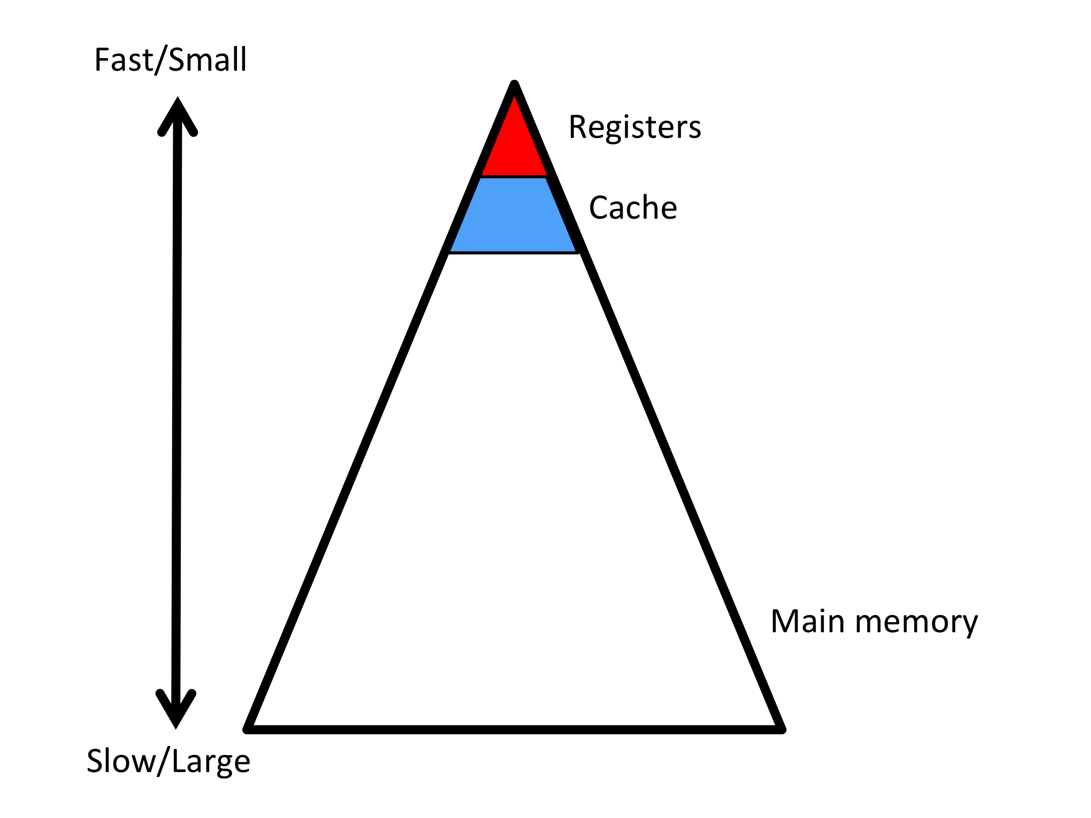
• That core has three levels of memory: registers, a cache memory, and main memory.

  

• Moving data between the cache and registers takes time \(\beta_{C\leftrightarrow R} \) per double while moving it between main memory and the cache takes time \(\beta_{M\leftrightarrow C} \)

• The registers can hold 64 doubles.

• The cache memory can hold one or more smallish matrices.

• Performing a floating point operation (multiply or add) with data in cache takes time \(\gamma_C \text{.}\)

• Data movement and computation cannot overlap. (In practice, it can. For now, we keep things simple.)

The idea now is to figure out how to block the matrices into submatrices and then compute while these submatrices are in cache to avoid having to access memory more than necessary.

A naive approach partitions \(C \text{,}\) \(A \text{,}\) and \(B \) into (roughly) square blocks:

and

where \(C_{i,j} \) is \(m_C \times n_C \text{,}\) \(A_{i,p} \) is \(m_C \times k_C \text{,}\) and \(B_{p,j} \) is \(k_C \times n_C \text{.}\) Then

which can be written as the triple-nested loop

This is one of \(3! = 6 \) possible loop orderings.

If we choose \(m_C\text{,}\) \(n_C \text{,}\) and \(k_C \) such that \(C_{i,j} \text{,}\) \(A_{i,p} \text{,}\) and \(B_{p,j} \) all fit in the cache, then we meet our conditions. We can then compute \(C_{i,j} := A_{i,p} B_{p,j} + C_{i,j} \) by "bringing these blocks into cache" and computing with them before writing out the result, as before. The difference here is that while one can explicitly load registers, the movement of data into caches is merely encouraged by careful ordering of the computation, since replacement of data in cache is handled by the hardware, which has some cache replacement policy similar to "least recently used" data gets evicted.

#define MC 96
#define NC 96
#define KC 96

void MyGemm( int m, int n, int k, double *A, int ldA,
	     double *B, int ldB, double *C, int ldC )
{
  if ( m % MR != 0 || MC % MR != 0 ){
    printf( "m and MC must be multiples of MR\n" );
    exit( 0 );
  }
  if ( n % NR != 0 || NC % NR != 0 ){
    printf( "n and NC must be multiples of NR\n" );
    exit( 0 );
  }
  
  for ( int i=0; i<m; i+=MC ) {
    int ib = min( MC, m-i );        /* Last block may not be a full block */
    for ( int j=0; j<n; j+=NC ) {
      int jb = min( NC, n-j );        /* Last block may not be a full block */
      for ( int p=0; p<k; p+=KC ) {
        int pb = min( KC, k-p );        /* Last block may not be a full block */
        Gemm_JI_MRxNRKernel
          ( ib, jb, pb, &alpha( i,p ), ldA, &beta( p,j ), ldB, &gamma( i,j ), ldC );
      }
    }
  }
}

void Gemm_JI_MRxNRKernel( int m, int n, int k, double *A, int ldA,
                                  double *B, int ldB, double *C, int ldC )
{
  for ( int j=0; j<n; j+=NR ) /* n is assumed to be a multiple of NR */
    for ( int i=0; i<m; i+=MR ) /* m is assumed to be a multiple of MR */
      Gemm_MRxNRKernel( k, &alpha( i,0 ), ldA, &beta( 0,j ), ldB, &gamma( i,j ), ldC );
}

Homework 3.2.1.2.

In Figure 3.2.1, we give an IJP loop ordering around the computation of \(C_{i,j} := A_{i,p} B_{p,j} + C_{i,j} \text{,}\) which itself is implemented by Gemm_JI_4x4Kernel. It can be found in Assignments/Week3/C/Gemm_IJP_JI_MRxNRKernel.c. Copy Gemm_4x4Kernel.c from Week 2 into Assignments/Week3/C/ and then execute

make IJP_JI_4x4Kernel

in that directory. The resulting performance can be viewed with Live Script Assignments/Week3/C/data/Plot_XYZ_JI_MRxNRKernel.mlx.

Solution

On Robert's laptop:

Notice that now performance is (mostly) maintained as the problem size increases.

Homework 3.2.1.3.

You can similarly link Gemm_IJP_JI_MRxNRKernel.c with your favorite micro-kernel by copying it from Week 2 into this directory and executing

make IJP_JI_??x??Kernel

where ??x?? reflects the \(m_R \times n_R\) you choose. The resulting performance can be viewed with Live Script Assignments/Week3/C/data/Plot_XYZ_JI_MRxNRKernel.mlx, by making appropriate changes to that Live Script.

The Live Script assumes ??x?? to be 12x4. If you choose (for example) 8x6 instead, you may want to do a global "search and replace." You may then want to save the result into another file.

Solution

On Robert's laptop, for \(m_R \times n_R = 12 \times 4 \text{:}\)

Homework 3.2.1.4.

Create all six loop orderings by copying Assignments/Week3/C/Gemm_IJP_JI_MRxNRKernel.c into

Gemm_JIP_JI_MRxNRKernel.c 
Gemm_IPJ_JI_MRxNRKernel.c 
Gemm_PIJ_JI_MRxNRKernel.c 
Gemm_PJI_JI_MRxNRKernel.c 
Gemm_JPI_JI_MRxNRKernel.c

(or your choice of \(m_R\) and \(n_R\)), reordering the loops as indicated by the XYZ. Collect performance data by executing

make XYZ_JI_12x4Kernel

for \({\tt XYZ} \in \{ {\tt IPJ},{\tt JIP},{\tt JPI},{\tt PIJ},{\tt PJI} \} \text{.}\)

(If you don't want to do them all, implement at least Gemm_PIJ_JI_MRxNRKernel.c.)

The resulting performance can be viewed with Live Script Assignments/Week3/C/data/Plot_XYZ_JI_MRxNRKernel.mlx.

Solution

• Assignments/Week3/Answers/Gemm_IPJ_JI_MRxNRKernel.c

• Assignments/Week3/Answers/Gemm_JIP_JI_MRxNRKernel.c

• Assignments/Week3/Answers/Gemm_JPI_JI_MRxNRKernel.c

• Assignments/Week3/Answers/Gemm_PIJ_JI_MRxNRKernel.c

• Assignments/Week3/Answers/Gemm_PJI_JI_MRxNRKernel.c

On Robert's laptop, for \(m_R \times n_R = 12 \times 4 \text{:}\)

Things are looking up!

We can analyze the cost of moving submatrices \(C_{i,j} \text{,}\) \(A_{i,p} \text{,}\) and \(B_{p,j} \) into the cache and computing with them:

which equals

Hence, the ratio of time spent in useful computation and time spent in moving data between main memory a cache is given by

Another way of viewing this is that the ratio between the number of floating point operations and number of doubles loaded/stored is given by

If, for simplicity, we take \(m_C = n_C = k_C = b \) then we get that

Thus, the larger \(b \text{,}\) the better the cost of moving data between main memory and cache is amortized over useful computation.

Above, we analyzed the cost of computing with and moving the data back and forth between the main memory and the cache for computation with three blocks (a \(m_C \times n_C\) block of \(C\text{,}\) a \(m_C \times k_C\) block of \(A\text{,}\) and a \(k_C \times n_C\) block of \(B\)). If we analyze the cost of naively doing so with all the blocks, we get

What this means is that the effective ratio is the same if we consider the entire computation \(C := A B + C \text{:}\)