Unit 3.2.3 Which cache to target?
Homework 3.2.3.1.
In Assignments/Week3/C, execute
make PI_JI_12x4_MCxKCand view the performance results with Live Script
Assignments/Week3/C/data/Plot_MC_KC_Performance.mlx.
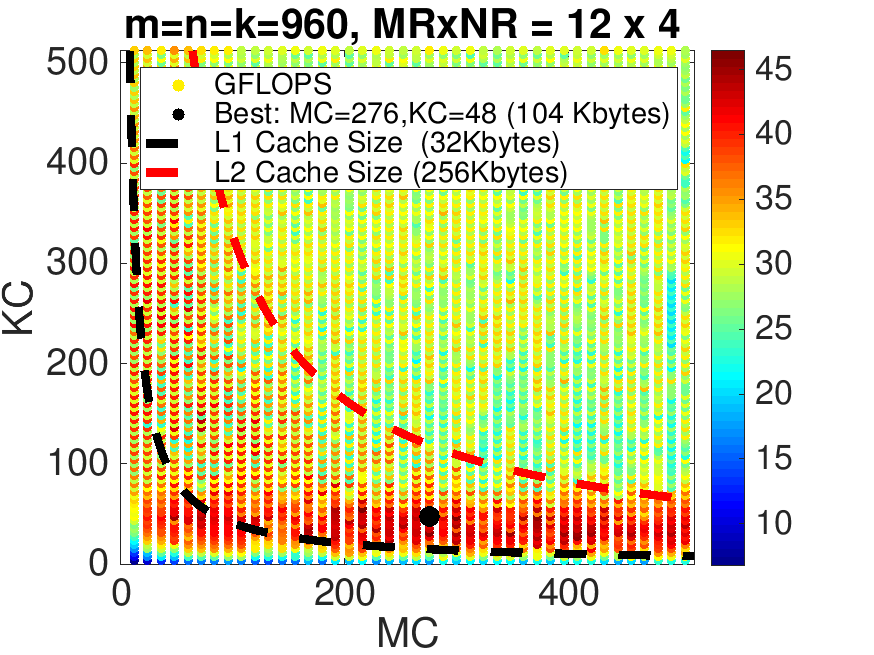
This experiment tries many different choices for \(m_C \) and \(k_C \text{,}\) and presents them as a scatter graph so that the optimal choice can be determined and visualized.
It will take a long time to execute. Go take a nap, catch a movie, and have some dinner! If you have a relatively old processor, you may even want to run it over night. Try not to do anything else on your computer, since that may affect the performance of an experiment. We went as far as to place something under the laptop to lift it off the table, to improve air circulation. You will notice that the computer will start making a lot of noise, as fans kick in to try to cool the core.
The last homework on Robert's laptop yields the performance in Figure 3.2.8.
To summarize, our insights suggest
Bring an \(m_C \times k_C \) submatrix of \(A \) into the cache, at a cost of \(m_C \times k_C \beta_{M \leftrightarrow C} \text{,}\) or \(m_C \times k_C\) memory operations (memops). (It is the order of the loops and instructions that encourages the submatrix of \(A \) to stay in cache.) This cost is amortized over \(2 m_C n k_C\) flops for a ratio of \(2 m_C n k_C / (m_C k_C) = 2 n \text{.}\) The larger \(n \text{,}\) the better.
The cost of reading an \(k_C \times n_R \) submatrix of \(B \) is amortized over \(2 m_C n_R k_C \) flops, for a ratio of \(2 m_C n_R k_C / ( k_C n_R) = 2 m_C \text{.}\) Obviously, the greater \(m_C \text{,}\) the better.
The cost of reading and writing an \(m_R \times n_R \) submatrix of \(C \) is now amortized over \(2 m_R n_R k_C \) flops, for a ratio of \(2 m_R n_R k_C / ( 2 m_R n_R) = k_C \text{.}\) Obviously, the greater \(k_C \text{,}\) the better.
Item 2 and Item 3 suggest that \(m_C \times k_C \) submatrix \(A_{i,p} \) be squarish.
If we revisit the performance data plotted in Figure 3.2.8, we notice that matrix \(A_{i,p} \) fits in part of the L2 cache, but is too big for the L1 cache. What this means is that the cost of bringing elements of \(A\) into registers from the L2 cache is low enough that computation can offset that cost. Since the L2 cache is larger than the L1 cache, this benefits performance, since the \(m_C \) and \(k_C \) can be larger.