Unit 4.1.1 Launch
¶In this launch, you get a first exposure to parallelizing implementations of matrix-matrix multiplication with OpenMP. By examining the resulting performance data in different ways, you gain a glimpse into how to interpret that data.
Recall how the IJP ordering can be explained by partitioning matrices: Starting with \(C := A B + C \text{,}\) partitioning \(C \) and \(A \) by rows yields
What we recognize is that the update of each row of \(C \) is completely independent and hence their computation can happen in parallel.
Now, it would be nice to simply tell the compiler "parallelize this loop, assigning the iterations to cores in some balanced fashion." For this, we use a standardized interface, OpenMP, to which you will be introduced in this week.
For now, all you need to know is:
You need to include the header file omp.h
#include "omp.h"
at the top of a routine that uses OpenMP compiler directives and/or calls to OpenMP routines and functions.You need to insert the line
#pragma omp parallel for
before the loop the iterations of which can be executed in parallel.You need to set the environment variable OMP_NUM_THREADS to the number of threads to be used in parallel
export OMP_NUM_THREADS=4
before executing the program.
The compiler blissfully does the rest.
Remark 4.1.1.
In this week, we get serious about collecting performance data. You will want to
Make sure a laptop you are using is plugged into the wall, since running on battery can do funny things to your performance.
Close down browsers and other processes that are running on your machine. I noticed that Apple's Activity Monitor can degrade performance a few percent.
Learners running virtual machines will want to assign enough virtual CPUs.
Homework 4.1.1.1.
In Assignments/Week4/C/ execute
export OMP_NUM_THREADS=1
make IJP
to collect fresh performance data for the IJP loop ordering.
Next, copy Gemm_IJP.c to Gemm_MT_IJP.c. (MT for Multithreaded). Include the header file omp.h at the top and insert the directive discussed above before the loop indexed with i. Compile and execute with the commands
export OMP_NUM_THREADS=4
make MT_IJP
ensuring only up to four cores are used by setting OMP_NUM_THREADS=4. Examine the resulting performance with the Live Script data/Plot_MT_Launch.mlx.
You may want to vary the number of threads you use depending on how many cores your processor has. You will then want to modify that number in the Live Script as well.
Homework 4.1.1.2.
In Week 1, you discovered that the JPI ordering of loops yields the best performance of all (simple) loop orderings. Can the outer-most loop be parallelized much like the outer-most loop of the IJP ordering? Justify your answer. If you believe it can be parallelized, in Assignments/Week4/C/ execute
make JPIto collect fresh performance data for the JPI loop ordering.
Next, copy Gemm_JPI.c to Gemm_MT_JPI.c. Include the header file omp.h at the top and insert the directive discussed above before the loop indexed with j. Compile and execute with the commands
export OMP_NUM_THREADS=4
make MT_JPI
Examine the resulting performance with the Live Script data/Plot_MT_Launch.mlx by changing ( 0 ) to ( 1 ) (in four places).
The loop ordering JPI also allows for convenient parallelization of the outer-most loop. Partition \(C\) and \(B\) by columns. Then
This illustrates that the columns of \(C\) can be updated in parallel.
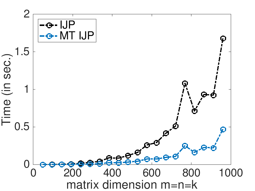
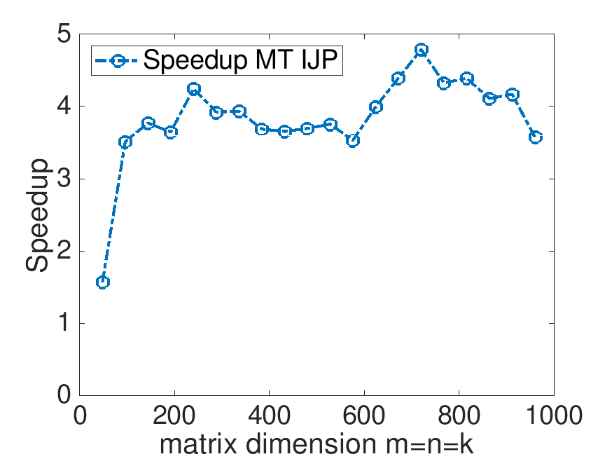
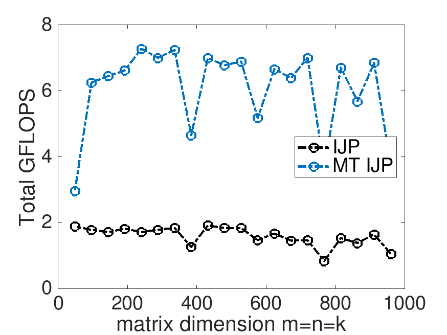
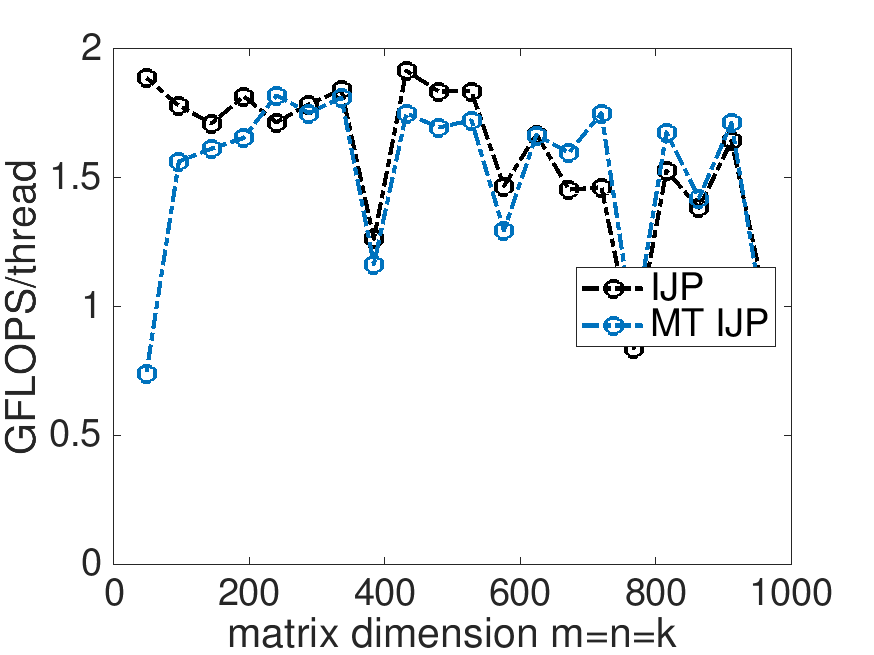
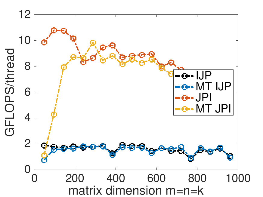
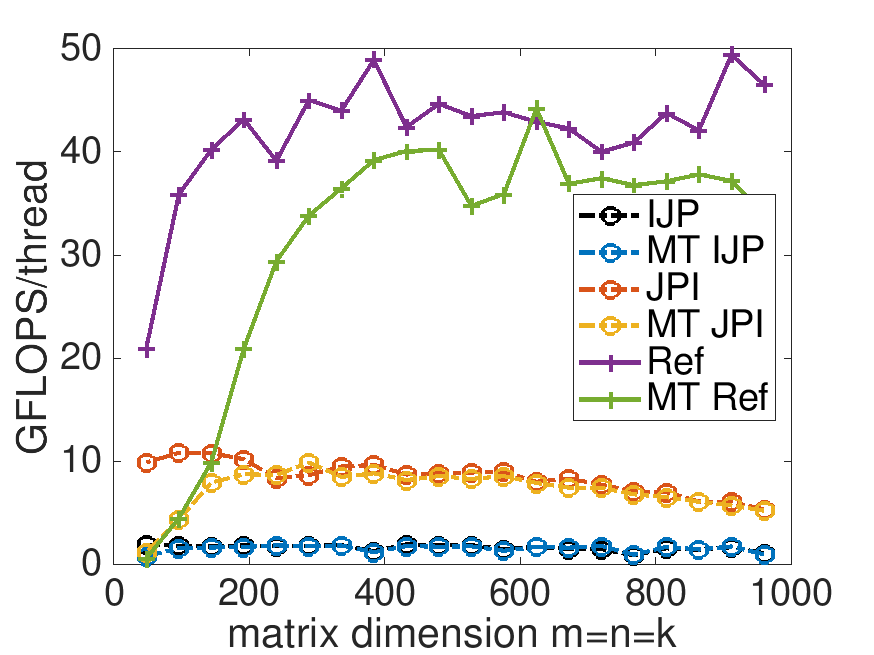
On Robert's laptop (using 4 threads):
Time:
Speedup
Total GFLOPS
GFLOPS per thread
Homework 4.1.1.3.
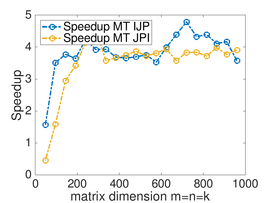
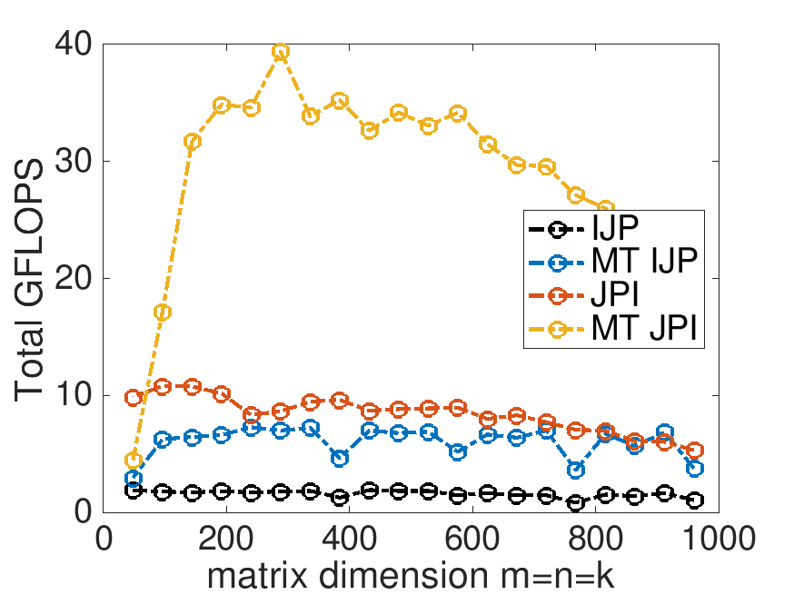
With Live Script data/Plot_MT_Launch.mlx, modify Plot_MT_Launch.mlx, by changing ( 0 ) to ( 1 ) (in four places), so that the results for the reference implementation are also displayed. Which multithreaded implementation yields the best speedup? Which multithreaded implementation yields the best performance?
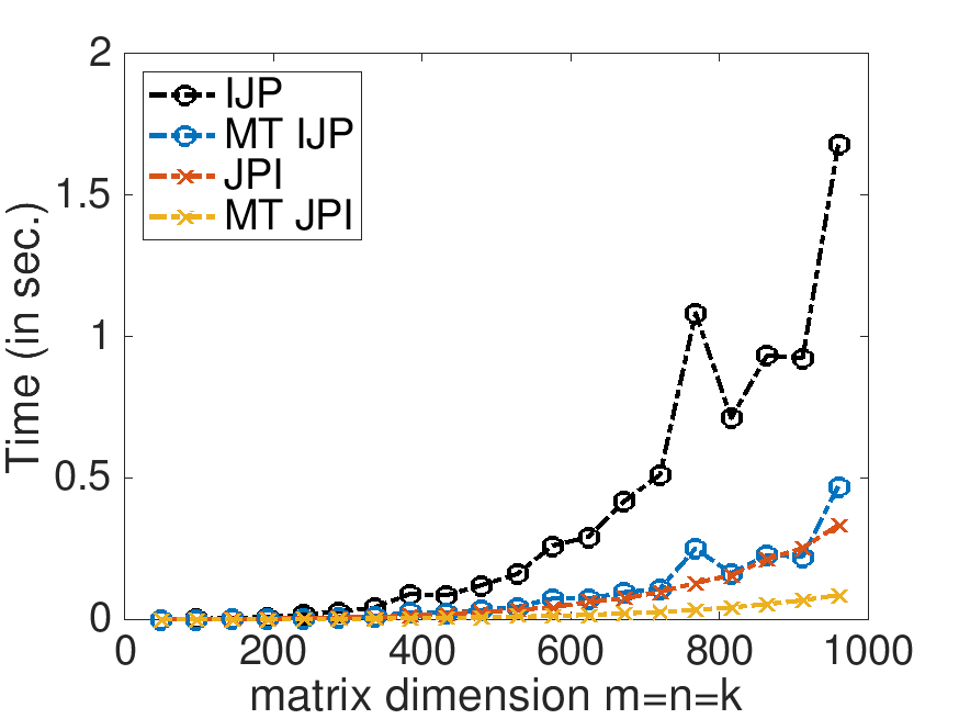
On Robert's laptop (using 4 threads):
Time:
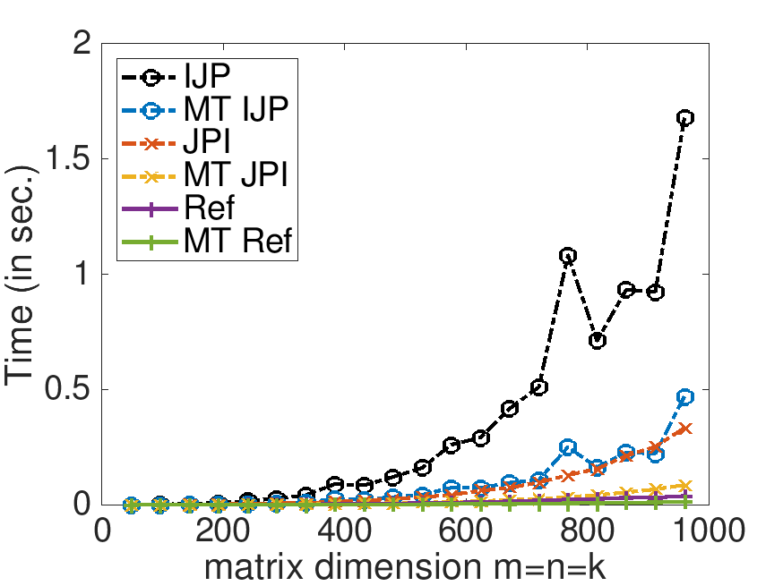
Speedup
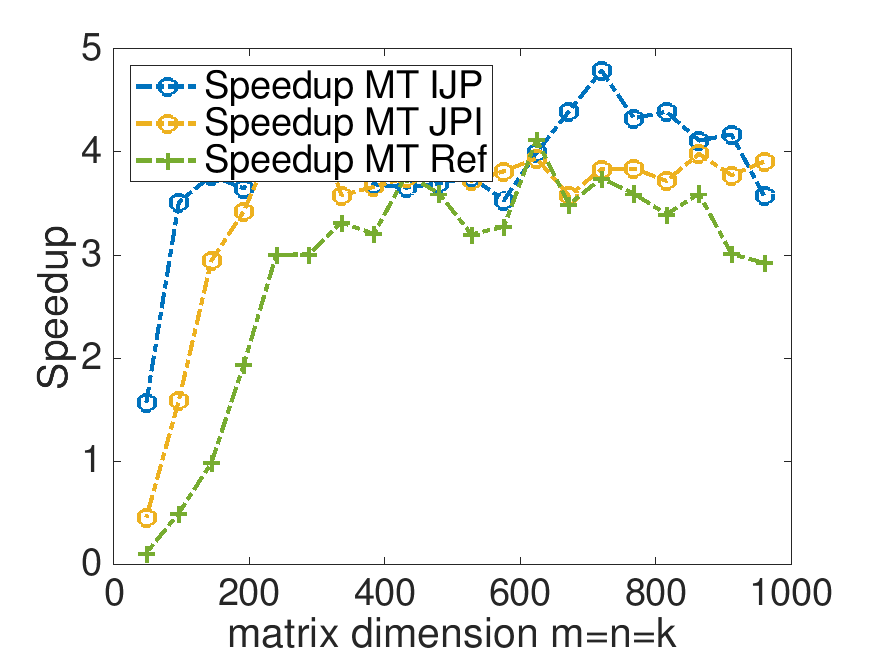
Total GFLOPS
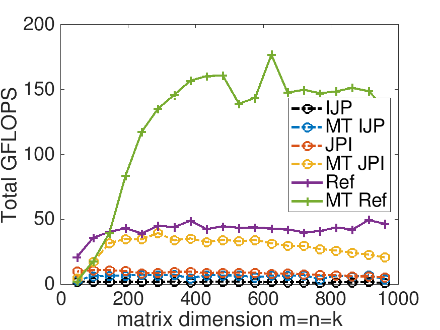
GFLOPS per thread
Remark 4.1.2.
In later graphs, you will notice a higher peak GFLOPS rate for the reference implementation. Up to this point in the course, I had not fully realized the considerable impact having other applications open on my laptop has on the performance experiments. we get very careful with this starting in Section 4.3.
Learn more:
For a general discussion of pragma directives, you may want to visit https://www.cprogramming.com/reference/preprocessor/pragma.html