Unit 3.4 More loop invariants
Neither of the loop invariants in (3.3) and (3.4) yield \({\bf Algorithm~5} \text{.}\) Perhaps there are even more loop invariants to be found.
Experience with deriving many algorithms for operations involving matrices and vectors has taught us that loop invariants can be derived best from purely recursive definitions of the operation. Let us illustrate this for our evaluation of a polynomial.
We start with
\begin{equation}
y = \sum_{i=0}^{k-1} a_i x^i + \sum_{i=k}^{n-1} a_i x^i
~\wedge ~ 0 \leq k \leq n,\label{SplitRange}\tag{3.5}
\end{equation}
which came from splitting the range. Next, we manipulate this expression:
\begin{equation*}
\begin{array}{l}
\sum_{i=0}^{k-1} a_i x^i + \sum_{i=k}^{n-1} a_i x^i
~\wedge ~ 0 \leq k \leq n \\
~~~ = ~~~~ \lt \mbox{definition of summation quantifier} \gt \\
\sum_{i=0}^{k-1} a_i x^i
+
\begin{array}[t]{c}
\underbrace{
a_k x^k + \cdots + a_{n-1} x^{n-1}
}
\\
\sum_{i=k}^{n-1} a_i x^i
\end{array}
~\wedge ~ 0 \leq k \leq n
\\
~~~ = ~~~~ \lt \mbox{factor out } x^ k \gt \\
\sum_{i=0}^{k-1} a_i x^i
+
\begin{array}[t]{c}
\underbrace{
\left(a_k x^{k-k} + \cdots + a_{n-1} x^{n-1-k} \right) x^k
}
\\
\left( \sum_{i=k}^{n-1} a_i x^{i-k} \right) x^k
\end{array}
~\wedge ~ 0 \leq k \leq n
\\
~~~ = ~~~~ \lt \mbox{reintroduce the summation quantifier} \gt \\
\sum_{i=0}^{k-1} a_i x^i + \left(\sum_{i=k}^{n-1} a_i x^{i-k}\right) x^k ~\wedge ~ 0 \leq k \leq n \\
~~~ = ~~~~ \lt \mbox{introduce new variable to keep track of } x^k
\gt \\
\sum_{i=0}^{k-1} a_i x^i + \left(\sum_{i=k}^{n-1} a_i x^{i-k}\right) z ~\wedge z = x^k ~\wedge ~ 0 \leq k \leq n
\end{array}
\end{equation*}
This yields the alternative expression for (3.5) given by
\begin{equation}
y = \sum_{i=0}^{k-1} a_i x^i + \left(\sum_{i=k}^{n-1} a_i x^{i-k}\right) z ~\wedge z = x^k ~\wedge ~ 0 \leq k \leq n \label{AlternativePME}\tag{3.6}
\end{equation}
from which we can derive five loop invariants:
\begin{equation*}
\begin{array}{| l | l |} \hline
{\bf Invariant~1} \amp
y = \sum_{i=0}^{k-1} a_i x^i \phantom{ +
\left(\sum_{i=k}^{n-1} a_i x^{i-k}\right) z ~\wedge z = x^k
~} \wedge ~ 0 \leq k \leq n
\\ \hline
{\bf Invariant~2} \amp
y = \sum_{i=0}^{k-1} a_i x^i \phantom{ +
\left(\sum_{i=k}^{n-1} a_i x^{i-k}\right) z }~\wedge z = x^k
~\wedge ~ 0 \leq k \leq n
\\ \hline
{\bf Invariant~3} \amp
\phantom{ y = \sum_{i=0}^{k-1} a_i x^i + }
\left(\sum_{i=k}^{n-1} a_i x^{i-k}\right) x^k ~ \phantom{\wedge z = x^k }
~\wedge ~ 0 \leq k \leq n
\\ \hline
{\bf Invariant~4} \amp
y = \sum_{i=0}^{k-1} a_i x^i {\color{lightgray!50} +
\left(\sum_{i=k}^{n-1} a_i x^{i-k}\right) z }~\wedge z = x^k
~\wedge ~ 0 \leq k \leq n
\\ \hline
{\bf Invariant~5} \amp
y =
\phantom{\sum_{i=0}^{k-1} a_i x^i + }
\left(\sum_{i=k}^{n-1} a_i x^{i-k}\right) \phantom{z ~\wedge z =
x^k }
~\wedge ~ 0 \leq k \leq n \\
\hline
\end{array}
\end{equation*}
We recognize that \({\bf Invariant~1} \) yields \({\bf
Algorithm~1} \) and \({\bf Invariant~3} \) is equivalent to the loop invariant in (3.4) and hence yields \({\bf
Algorithm~3} \text{.}\)
Exercise 3.2.
Derive \({\bf Algorithm~2} \) that responding \({\bf Invariant~2} \text{.}\) Explicitly introduce \(z \) as a variable in the program.
A comment regarding \({\bf Invariant~3} \) is in order since it does not follow from (3.6) by removing terms. One can view that invariant alternatively as
\begin{equation*}
y = \sum_{i=0}^{k-1} a_i x^i {\color{lightgray!50} +
\left(\sum_{i=k}^{n-1} a_i x^{i-k}\right) z }~\wedge z = x^k
~\wedge ~ 0 \leq k \leq n,
\end{equation*}
which is \({\bf Invariant~4} \text{,}\) where the \(z \) is introduced as a dummy variable. By this we mean that it occurs in the assertions in the program rather than as an actual variable in the commands of the program.
Exercise 3.3.
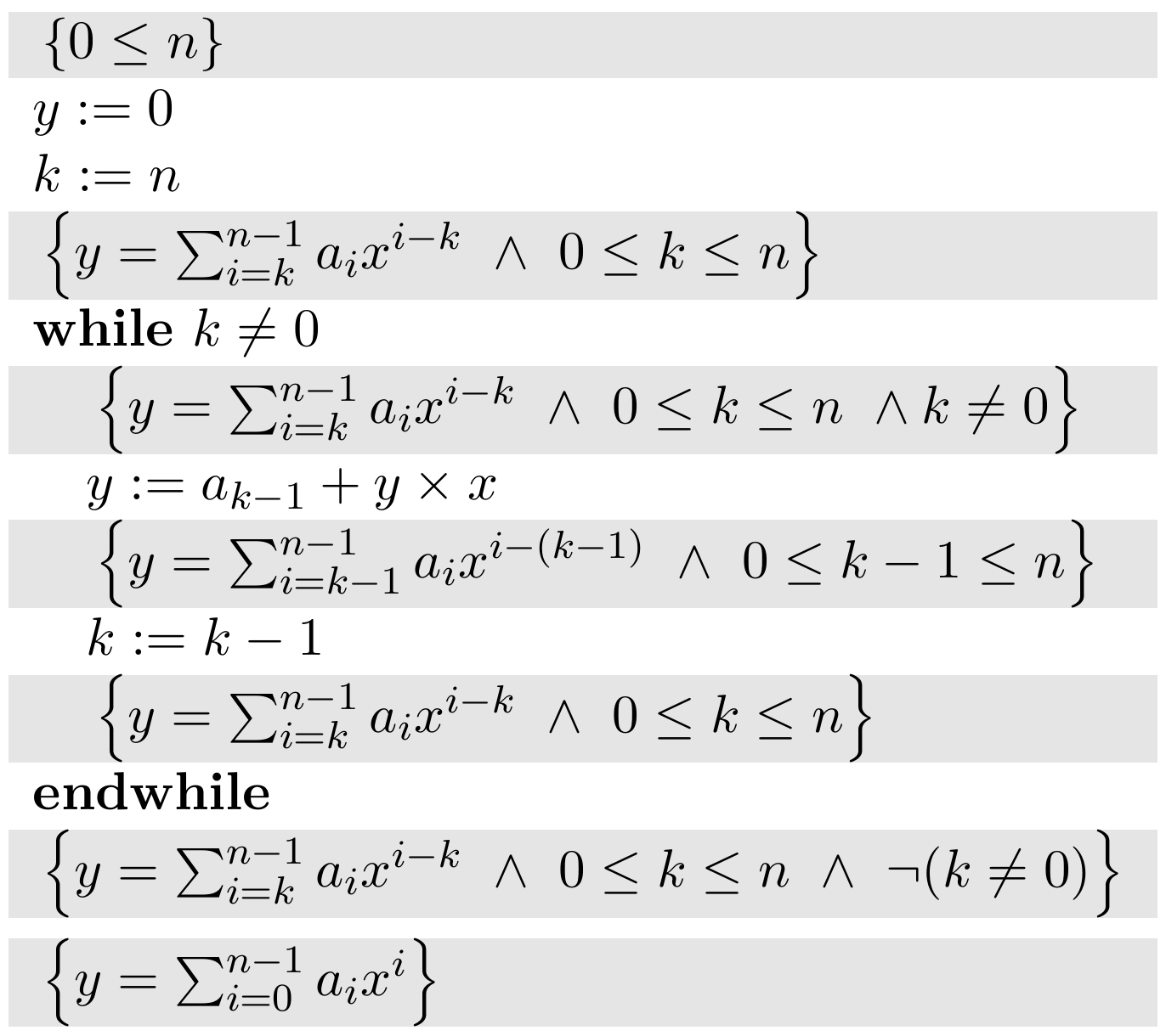
Derive \({\bf Algorithm~5} \) that responding \({\bf Invariant~5} \text{.}\) No not introduce \(z \) as a variable in the program.
\({\bf Algorithm~5} \) is known as Horner's rule and can be explained by observing that
\begin{equation*}
\begin{array}{rcl}
y
\amp =\amp
a_0 + a_1 x + a_2 x^2 + \cdots + a_{n-1} x^{n-1}\\
\amp = \amp
a_0 + (a_1 + (a_2 + ( \cdots + a_{n-1} x ) \cdots ) x ) x .
\end{array}
\end{equation*}
The algorithm evaluates the expression in a way that obeys the parentheses.
We conclude by observing that (3.6) is a recursive definition of the operation:
\begin{equation*}
y = \sum_{i=0}^{k-1} a_i x^i + \left(\sum_{i=k}^{n-1} a_i x^{i-k}\right) z ~\wedge z = x^k ~\wedge ~ 0 \leq k \leq n
\end{equation*}
can be rewritten as
\begin{equation*}
y = \sum_{i=0}^{k-1} a_i x^i + \left(\sum_{i=0}^{n-1-k} a_{i+k} x^{i}\right) z ~\wedge z = x^k ~\wedge ~ 0 \leq k \leq n
\end{equation*}
where
\(\sum_{i=0}^{k-1} a_i x^i \) is a polynomial of degree \(k-1 \) defined by the coefficients \(a_0,
\ldots , a_{k-1} \) and
\(\sum_{i=0}^{n-1-k} a_{i+k} x^i \) is a polynomial of degree \(n-1-k \) defined by the coefficients \(a_k,
\ldots , a_{n-1} \text{.}\)
Thus, our systematic methodology turns a recursive definition of an operation into a loop-based program, via the systematic discovery of loop invariants.
Exercise 3.4.
Compare and contrast the five different algorithms. Which one is the "best"?