
Section 1.4 Thinking in Terms of Matrix-Vector Operations

Unit 1.4.1 Matrix-vector multiplication via dot products or axpy operations

Homework 1.4.1

Compute \(\left(\begin{array}{rrrr} 2 \amp 2 \amp -1 \amp 2\\ 2 \amp 1 \amp 0 \amp -2\\ -2 \amp -2 \amp 2 \amp 2 \end{array}\right) \left(\begin{array}{r} 2\\ -1\\ 0\\ -1 \end{array}\right) =\)

Solution
\(\left(\begin{array}{rrrr} 2 \amp 2 \amp -1 \amp 2\\ \hline 2 \amp 1 \amp 0 \amp -2\\ \hline -2 \amp -2 \amp 2 \amp 2 \end{array}\right) \left(\begin{array}{r} 2\\ -1\\ 0\\ -1 \end{array}\right) = \left( \begin{array}{r} \left(\begin{array}{rrrr} 2 \amp 2 \amp -1 \amp 2 \end{array}\right) \left(\begin{array}{r} 2\\ -1\\ 0\\ -1 \end{array}\right) \\ \hline \left(\begin{array}{rrrr} 2 \amp 1 \amp 0 \amp -2 \end{array}\right) \left(\begin{array}{c} 2\\ -1\\ 0\\ -1 \end{array}\right) \\ \hline \left(\begin{array}{rrrr} -2 \amp -2 \amp 2 \amp 2 \end{array}\right) \left(\begin{array}{c} 2\\ -1\\ 0\\ -1 \end{array}\right) \end{array} \right)\)

Consider the matrix-vector multiplication (MVM)

\begin{equation*} y := A x + y . \end{equation*}

The way one is usually taught to compute this operations is that each element of \(y \text{,}\) \(\psi_i \text{,}\) is updated with the dot product of the corresponding row of \(A \text{,}\) \(\widetilde a_i^T \text{,}\) with vector \(x \text{.}\) With our notation, we can describe this as

\begin{equation*} \begin{array}{rcl} \left( \begin{array}{c} \psi_0 \\ \hline \psi_1 \\ \hline \vdots \\ \hline \psi_{m-1} \end{array} \right) := \left( \begin{array}{c} \widetilde a_0^T \\ \hline \widetilde a_1^T \\ \hline \vdots \\ \hline \widetilde a_{m-1}^T \end{array} \right) x + \left( \begin{array}{c} \psi_0 \\ \hline \psi_1 \\ \hline \vdots \\ \hline \psi_{m-1} \end{array} \right) = \left( \begin{array}{c} \widetilde a_0^T x + \psi_0 \\ \hline \widetilde a_1^T x + \psi_1 \\ \hline \vdots \\ \hline \widetilde a_{m-1}^T x + \psi_{m-1} \end{array} \right). \end{array} \end{equation*}

If we then expose the individual elements of \(A \) and \(y \) we get

\begin{equation*} \begin{array}{l} \left( \begin{array}{c} \psi_0 \\ \psi_1 \\ \vdots \\ \psi_{m-1} \end{array}\right) \\ ~~~:= \left( \begin{array}{c @{~} c @{~} c @{~} c @{~} c @{~} c @{~} c @{~} c @{~} c @{~} c @{~} c} \alpha_{0,0} \amp \chi_0 \amp + \amp \alpha_{0,1} \amp \chi_1 \amp + \amp \cdots \amp \alpha_{0,n-1} \amp \chi_{n-1} \amp+ \amp \psi_0 \\ \alpha_{1,0} \amp \chi_0 \amp + \amp \alpha_{1,1} \amp \chi_1 \amp + \amp \cdots \amp \alpha_{1,n-1} \amp \chi_{n-1} \amp + \amp \psi_1 \\ \amp\amp\amp\amp\amp\vdots\amp\amp\amp \\ \alpha_{m-1,0} \amp \chi_0 \amp + \amp \alpha_{m-1,1} \amp \chi_1 \amp + \amp \cdots \amp \alpha_{m-1,n-1} \amp \chi_{n-1} \amp + \amp \psi_{m-1} \end{array} \right) \\ ~~~= \left( \begin{array}{c @{~} c @{~} c @{~} c @{~} c @{~} c @{~} c @{~} c @{~} c @{~} c @{~} c} \chi_0 \amp \alpha_{0,0} \amp + \amp \chi_1 \amp \alpha_{0,1} \amp + \amp \cdots \amp \chi_{n-1} \amp \alpha_{0,n-1} \amp + \amp \psi_0 \\ \chi_0 \amp \alpha_{1,0} \amp + \amp \chi_1 \amp \alpha_{1,1} \amp + \amp \cdots \amp \chi_{n-1} \amp \alpha_{1,n-1} \amp + \amp \psi_1 \\ \amp\amp\amp\amp\amp\vdots\amp\amp\amp \\ \chi_0 \amp \alpha_{m-1,0} \amp + \amp \chi_1 \amp \alpha_{m-1,1} \amp + \amp \cdots \amp \chi_{n-1} \amp \alpha_{m-1,n-1} \amp + \amp \psi_{m-1} \end{array} \right) \end{array} \end{equation*}

This discussion explains the IJ loop for computing \(y := A x + y \text{:}\)

\begin{equation*} \begin{array}{l} {\bf for~} i := 0, \ldots , m-1 \\[0.05in] ~~~ \left. \begin{array}{l} {\bf for~} j := 0, \ldots , n-1 \\ ~~~ ~~~ \psi_i := \alpha_{i,j} \chi_{j} + \psi_i \\ {\bf end} \end{array} \right\} ~~~ \psi_i := \widetilde a_j^T x + \psi_i \\[0.1in] {\bf end} \end{array} \end{equation*}

What it demonstrates is how matrix-vector multiplication can be implemented as a sequence of dot operations.

Homework 1.4.2

In directory Assignments/Week1/C complete the implementation of matrix-vector multiplication in terms of dot operations

#define alpha( i,j ) A[ (j)*ldA + i ]   // map alpha( i,j ) to array A 
#define chi( i )  x[ (i)*incx ]         // map chi( i )  to array x
#define psi( i )  y[ (i)*incy ]         // map psi( i )  to array x

void Dots( int, const double *, int, const double *, int, double * );

void Gemv( int m, int n, double *A, int ldA,
           double *x, int incx, double *y, int incy )
{
  for ( int i=0; i<m; i++ )
    Dots(   ,      ,     ,     ,    ,      );
}

in file Assignments/Week1/C/Gemv_I_Dots.c. You will test this with an implementation of matrix-matrix multiplication in a later homework.

Next, partitioning \(m \times n \) matrix \(A \) by columns and \(x \) by individual elements, we find that

\begin{equation*} \begin{array}{rcl} y \amp:=\amp \left( \begin{array}{c | c | c | c} a_0 \amp a_1 \amp \cdots \amp a_{n-1} \end{array} \right) \left( \begin{array}{c} \chi_0 \\ \hline \chi_1 \\ \hline \vdots \\ \hline \chi_{n-1} \end{array} \right) + y \\ \amp=\amp \chi_0 a_0 + \chi_1 a_1 + \cdots + \chi_{n-1} a_{n-1} + y. \end{array} \end{equation*}

If we then expose the individual elements of \(A \) and \(y \) we get

\begin{equation*} \begin{array}{l} \left( \begin{array}{c} \psi_0 \\ \psi_1 \\ \vdots \\ \psi_{m-1} \end{array}\right) \\ ~~~:= \chi_0 \left( \begin{array}{c} \alpha_{0,0} \\ \alpha_{1,0} \\ \vdots \\ \alpha_{m-1,0} \end{array}\right) + \chi_1 \left( \begin{array}{c} \alpha_{0,1} \\ \alpha_{1,1} \\ \vdots \\ \alpha_{m-1,1} \end{array}\right) + \cdots + \chi_{n-1} \left( \begin{array}{c} \alpha_{0,n-1} \\ \alpha_{1,n-1} \\ \vdots \\ \alpha_{m-1,n-1} \end{array}\right) + \left( \begin{array}{c} \psi_0 \\ \psi_1 \\ \vdots \\ \psi_{m-1} \end{array}\right) \\ ~~~= \left( \begin{array}{c @{~} c @{~} c @{~} c @{~} c @{~} c @{~} c @{~} c @{~} c @{~} c @{~} c} \chi_0 \amp \alpha_{0,0} \amp + \amp \chi_1 \amp \alpha_{0,1} \amp + \amp \cdots \amp \chi_{n-1} \amp \alpha_{0,n-1} \amp + \amp \psi_0 \\ \chi_0 \amp \alpha_{1,0} \amp + \amp \chi_1 \amp \alpha_{1,1} \amp + \amp \cdots \amp \chi_{n-1} \amp \alpha_{1,n-1} \amp + \amp \psi_1 \\ \amp\amp\amp\amp\amp\vdots\amp\amp\amp \\ \chi_0 \amp \alpha_{m-1,0} \amp + \amp \chi_1 \amp \alpha_{m-1,1} \amp + \amp \cdots \amp \chi_{n-1} \amp \alpha_{m-1,n-1} \amp + \amp \psi_{m-1} \end{array} \right). \end{array} \end{equation*}

This discussion explains the JI loop for computing \(y := A x + y \text{:}\)

\begin{equation*} \begin{array}{l} {\bf for~} j := 0, \ldots , n-1 \\ ~~~ \left. \begin{array}{l} {\bf for~} i := 0, \ldots , m-1 \\ ~~~ ~~~ \psi_i := \alpha_{i,j} \chi_{j} + \psi_i \\ {\bf end} \end{array} \right\} ~~~ y := \chi_j a_j + y \\[0.1in] {\bf end} \end{array} \end{equation*}

What it also demonstrates is how matrix-vector multiplication can be implemented as a sequence of axpy operations.

Homework 1.4.3

In directory Assignments/Week1/C complete the implementation of matrix-vector multiplication in terms of axpy operations

#define alpha( i,j ) A[ (j)*ldA + i ]   // map alpha( i,j ) to array A 
#define chi( i )  x[ (i)*incx ]         // map chi( i )  to array x
#define psi( i )  y[ (i)*incy ]         // map psi( i )  to array x

void Axpy( int, double, double *, int, double *, int );

void Gemv( int m, int n, double *A, int ldA,
           double *x, int incx, double *y, int incy )
{
  for ( int j=0; j<n; j++ )
    Axpy(  ,     ,      ,   ,   ,     );
}

in file Assignments/Week1/C/Gemv_J_Axpy.c. You will test this with an implementation of matrix-matrix multiplication in a later homework.

Unit 1.4.2 Matrix-matrix multiplication via matrix-vector multiplications

Homework 1.4.4

Fill in the blanks:

Figure 1.4.1 Click here to enlarge

Now that we are getting comfortable with partitioning matrices and vectors, we can view the six algorithms for \(C := A B + C \) is a more layered fashion. If we partition \(C \) and \(B \) by columns, we find that

\begin{equation*} \begin{array}{rcl} \left( \begin{array}{c | c | c | c } c_0 \amp c_1 \amp \cdots \amp c_{n-1} \end{array} \right) \amp:=\amp A \left( \begin{array}{c | c | c | c } b_0 \amp b_1 \amp \cdots \amp b_{n-1} \end{array} \right) + \left( \begin{array}{c | c | c | c } c_0 \amp c_1 \amp \cdots \amp c_{n-1} \end{array} \right) \\ \amp = \amp \left( \begin{array}{c | c | c | c } A b_0 + c_0 \amp A b_1 + c_1 \amp \cdots \amp A b_{n-1} + c_{n-1} \end{array} \right) \end{array} \end{equation*}

A picture that captures this is given by

This illustrates how the JIP and JPI algorithms can be viewed as a loop around matrix-vector multiplications:

\begin{equation*} \begin{array}{l} \begin{array}{l} {\bf for~} j := 0, \ldots , n-1 \\[0.15in] ~~~ \left. \begin{array}{l} {\bf for~} p := 0, \ldots , k-1 \\[0.15in] ~~~ ~~~ \left. \begin{array}{l} {\bf for~} i := 0, \ldots , m-1 \\ ~~~ ~~~ \gamma_{i,j} := \alpha_{i,p} \beta_{p,j} + \gamma_{i,j} \\ {\bf end} \end{array} \right\} ~~~ c_j := \beta_{p,j} a_p + c_j \\[0.2in] ~~~ {\bf end} \end{array} \right\} ~~~ c_j := A b_j + c_j \\[0.2in] {\bf end} \end{array} \end{array} \end{equation*}

and

\begin{equation*} \begin{array}{l} \begin{array}{l} {\bf for~} j := 0, \ldots , n-1 \\[0.15in] ~~~ \left. \begin{array}{l} {\bf for~} i := 0, \ldots , m-1 \\[0.15in] ~~~ ~~~ \left. \begin{array}{l} {\bf for~} p := 0, \ldots , k-1 \\ ~~~ ~~~ \gamma_{i,j} := \alpha_{i,p} \beta_{p,j} + \gamma_{i,j} \\ {\bf end} \end{array} \right\} ~~~ \gamma_{i,j} := \widetilde a_i^T b_j + \gamma_{i,j} \\[0.2in] ~~~ {\bf end} \end{array} \right\} ~~~ c_j := A b_j + c_j \\[0.2in] {\bf end} \end{array} \end{array} \end{equation*}

The BLAS include the routine dgemv that computes

\begin{equation*} y := \alpha A x + \beta y \quad \mbox{or} \quad y := \alpha A^T x + \beta y. \end{equation*}

If

  • \(m \times n \) matrix \(A \) is stored in array A with its leading dimension stored in variable ldA,

  • \(m \) is stored in variable m and \(n \) is stored in variable n,

  • vector \(x \) is stored in array x with its stride stored in variable incx,

  • vector \(y \) is stored in array y with its stride stored in variable incy, and

  • \(\alpha \) and \(\beta \) are stored in variables alpha and beta, respectively,

the \(y := \alpha A x + \beta y \) translates, from C, into the call

dgemv_( "No transpose", &m, &n, &alpha, A, &ldA, x, &incx,
           &beta, y, &incy );

The BLIS "native call" that is similar to the BLAS dgemv routine in this setting translates to

bli_dgemv( BLIS_NO_TRANSPOSE, BLIS_NO_CONJUGATE, m, n,
   &alpha, A, 1, ldA, x, incx, &beta, y, incy );

Notice the two parameters after A. BLIS requires a row and column stride to be specified for matrices, thus generalizing beyond column-major order storage.

Unit 1.4.3 Rank-1 update (rank-1)

An operation that is going to become very important in future discussion and optimization of \MMM\ is the rank-1 update:

\begin{equation*} A := x y^T + A . \end{equation*}
Homework 1.4.9

Compute \(\left(\begin{array}{r} 2\\ -1\\ 0 \end{array}\right) \left(\begin{array}{r r r r} -2 \amp 0 \amp 1 \amp -1 \end{array} \right) + \left(\begin{array}{rrrr} 2 \amp 2 \amp -1 \amp 2\\ 2 \amp 1 \amp 0 \amp -2\\ -2 \amp -2 \amp 2 \amp 2 \end{array}\right) =\)

Solution
\begin{equation*} \begin{array}{l} \left(\begin{array}{r} 2\\ -1\\ 0 \end{array}\right) \left(\begin{array}{r r r r} -2 \amp 0 \amp 1 \amp -1 \end{array} \right) + \left(\begin{array}{rrrr} 2 \amp 2 \amp -1 \amp 2\\ 2 \amp 1 \amp 0 \amp -2\\ -2 \amp -2 \amp 2 \amp 2 \end{array}\right) \\ ~~~ = \left(\begin{array}{rrrr} (2)(-2) \amp (2)(0) \amp (2)(1) \amp (2)(-1)\\ (-1)(-2) \amp (-1)(0) \amp (-1)(1) \amp (-1)(-1)\\ (0)(-2) \amp (0)(0) \amp (0)(1) \amp (0)(-1)\\ \end{array}\right) + \left(\begin{array}{rrrr} 2 \amp 2 \amp -1 \amp 2\\ 2 \amp 1 \amp 0 \amp -2\\ -2 \amp -2 \amp 2 \amp 2 \end{array}\right) \\ ~~~ = \left(\begin{array}{r|r|r|r} \left(\begin{array}{r} 2 \\ -1 \\ 0 \end{array} \right) (-2) \amp \left(\begin{array}{r} 2 \\ -1 \\ 0 \end{array} \right) (0) \amp \left(\begin{array}{r} 2 \\ -1 \\ 0 \end{array} \right) (1) \amp \left(\begin{array}{r} 2 \\ -1 \\ 0 \end{array} \right) (1) \end{array}\right) \\ ~~~~~ + \left(\begin{array}{r|r|r|r} 2 \amp 2 \amp -1 \amp 2\\ 2 \amp 1 \amp 0 \amp -2\\ -2 \amp -2 \amp 2 \amp 2 \end{array}\right) \\ ~~~ = \left(\begin{array}{r|r|r|r} (-2) \left(\begin{array}{r} 2 \\ -1 \\ 0 \end{array} \right) + \left(\begin{array}{r} 2 \\ 2 \\ -2 \end{array} \right) \amp (0) \left(\begin{array}{r} 2 \\ -1 \\ 0 \end{array} \right) + \left(\begin{array}{r} 2 \\ 1 \\ -2 \end{array} \right) \amp (1) \left(\begin{array}{r} 2 \\ -1 \\ 0 \end{array} \right) + \left(\begin{array}{r} -1 \\ 0 \\ 2 \end{array} \right) \amp (1) \left(\begin{array}{r} 2 \\ -1 \\ 0 \end{array} \right) + \left(\begin{array}{r} 2 \\ -2 \\ 2 \end{array} \right) \end{array}\right) \end{array} \end{equation*}

Also,

\begin{equation*} \begin{array}{l} \left(\begin{array}{r} 2\\ -1\\ 0 \end{array}\right) \left(\begin{array}{r r r r} -2 \amp 0 \amp 1 \amp -1 \end{array} \right) + \left(\begin{array}{rrrr} 2 \amp 2 \amp -1 \amp 2\\ 2 \amp 1 \amp 0 \amp -2\\ -2 \amp -2 \amp 2 \amp 2 \end{array}\right) \\ ~~~ = \left(\begin{array}{rrrr} (2)(-2) \amp (2)(0) \amp (2)(1) \amp (2)(-1)\\ (-1)(-2) \amp (-1)(0) \amp (-1)(1) \amp (-1)(-1)\\ (0)(-2) \amp (0)(0) \amp (0)(1) \amp (0)(-1)\\ \end{array}\right) + \left(\begin{array}{rrrr} 2 \amp 2 \amp -1 \amp 2\\ 2 \amp 1 \amp 0 \amp -2\\ -2 \amp -2 \amp 2 \amp 2 \end{array}\right) \\ ~~~ = \left(\begin{array}{r} (2) \left(\begin{array}{rrrr} -2 \amp 0 \amp 1 \amp -1 \end{array} \right) \\ \hline (-1) \left(\begin{array}{rrrr} -2 \amp 0 \amp 1 \amp -1 \end{array} \right) \\ \hline (0) \left(\begin{array}{rrrr} -2 \amp 0 \amp 1 \amp -1 \end{array} \right) \end{array}\right) \\ ~~~ + \left(\begin{array}{rrrr} 2 \amp 2 \amp -1 \amp 2\\ \hline 2 \amp 1 \amp 0 \amp -2\\ \hline -2 \amp -2 \amp 2 \amp 2 \end{array}\right) \\ ~~~ = \left(\begin{array}{r} (2) \left(\begin{array}{rrrr} -2 \amp 0 \amp 1 \amp -1 \end{array} \right) + \left(\begin{array}{rrrr} 2 \amp 2 \amp -1 \amp 2 \end{array} \right) \\ \hline (-1) \left(\begin{array}{rrrr} -2 \amp 0 \amp 1 \amp -1 \end{array} \right) + \left(\begin{array}{rrrr} 2 \amp 1 \amp 0 \amp -2 \end{array} \right) \\ \hline (0) \left(\begin{array}{rrrr} -2 \amp 0 \amp 1 \amp -1 \end{array} \right) + \left(\begin{array}{rrrr} -2 \amp -2 \amp 2 \amp 2 \end{array} \right) \end{array}\right) \end{array} \end{equation*}

Partitioning \(m \times n \) matrix \(A \) by columns, and \(x \) and \(y \) by individual elements, we find that

\begin{equation*} \begin{array}{l} \left(\begin{array}{c | c | c | c} \alpha_{0,0} \amp \alpha_{0,1} \amp \cdots \amp \alpha_{0,k-1} \\ \hline \alpha_{1,0} \amp \alpha_{1,1} \amp \cdots \amp \alpha_{1,k-1} \\ \hline \vdots \amp \vdots \amp \amp \vdots \\ \hline \alpha_{m-1,0} \amp \alpha_{m-1,1} \amp \cdots \amp \alpha_{m-1,k-1} \end{array} \right):= \\ \left( \begin{array}{c} \chi_0 \\ \hline \chi_1 \\ \hline \vdots \\ \hline \chi_{m-1} \end{array} \right) \left( \begin{array}{c | c | c | c} \psi_0 \amp \psi_1 \amp \cdots \amp \psi_{n-1} \end{array} \right) + \left(\begin{array}{c | c | c | c} \alpha_{0,0} \amp \alpha_{0,1} \amp \cdots \amp \alpha_{0,n-1} \\ \hline \alpha_{1,0} \amp \alpha_{1,1} \amp \cdots \amp \alpha_{1,n-1} \\ \hline \vdots \amp \vdots \amp \amp \vdots \\ \hline \alpha_{m-1,0} \amp \alpha_{m-1,1} \amp \cdots \amp \alpha_{m-1,n-1} \end{array} \right) \\ = \left(\begin{array}{c | c | c | c} \chi_0 \psi_0 + \alpha_{0,0} \amp \chi_0 \psi_1 + \alpha_{0,1} \amp \cdots \amp \chi_0 \psi_{n-1} + \alpha_{0,n-1} \\ \hline \chi_1 \psi_0 + \alpha_{1,0} \amp \chi_1 \psi_1 + \alpha_{1,1} \amp \cdots \amp \chi_1 \psi_{n-1} + \alpha_{1,n-1} \\ \hline \vdots \amp \vdots \amp \amp \vdots \\ \hline \chi_{m-1} \psi_0 + \alpha_{m-1,0} \amp \chi_{m-1} \psi_1 + \alpha_{m-1,1} \amp \cdots \amp \chi_{m-1} \psi_{n-1} + \alpha_{m-1,n-1} \end{array} \right) \\ = \left(\begin{array}{c | c | c | c} \left(\begin{array}{c} \chi_0 \\ \chi_1 \\ \vdots \\ \chi_{m-1} \end{array}\right) \psi_0 + \left(\begin{array}{c} \alpha_{0,0} \\ \alpha_{1,0} \\ \vdots \\ \alpha_{m-1,0} \end{array}\right) \amp \cdots \amp \left(\begin{array}{c} \chi_0 \\ \chi_1 \\ \vdots \\ \chi_{m-1} \end{array}\right) \psi_{n-1} + \left(\begin{array}{c} \alpha_{0,n-1} \\ \alpha_{1,n-1} \\ (\vdots \\ \alpha_{m-1,n-1} \end{array}\right) \end{array} \right) . \end{array} \end{equation*}

What this illustrates is that we could have partitioned \(A\) by columns and \(y \) by elements to find that

\begin{equation*} \begin{array}{l} \left(\begin{array}{c | c | c | c} a_0 \amp a_1 \amp \cdots \amp a_{n-1} \end{array} \right) \\ ~~~:= x \left( \begin{array}{c | c | c | c} \psi_0 \amp \psi_1 \amp \cdots \amp \psi_{n-1} \end{array} \right) + \left(\begin{array}{c | c | c | c} a_0 \amp a_1 \amp \cdots \amp a_{n-1} \end{array} \right) \\ ~~~= \left(\begin{array}{c | c | c | c} x \psi_0 + a_0 \amp x \psi_1 + a_1 \amp \cdots \amp x \psi_{n-1} + a_{n-1} \end{array} \right) \\ ~~~= \left(\begin{array}{c | c | c | c} \psi_0 x + a_0 \amp \psi_1 x + a_1 \amp \cdots \amp \psi_{n-1} x + a_{n-1} \end{array} \right). \end{array} \end{equation*}

This discussion explains the JI loop ordering for computing \(A := x y^T + A \text{:}\)

\begin{equation*} \begin{array}{l} {\bf for~} j := 0, \ldots , n-1 \\[0.05in] ~~~ \left. \begin{array}{l} {\bf for~} i := 0, \ldots , m-1 \\ ~~~ ~~~ \alpha_{i,j} := \chi_{i} \psi_{j} + \alpha_{i,j} \\ {\bf end} \end{array} \right\} ~~~ a_j := \psi_i x + a_j \\[0.1in] {\bf end} \end{array} \end{equation*}

What it also demonstrates is how the rank-1 operation can be implemented as a sequence of axpy operations.

Homework 1.4.10

In Assignments/Week1/C/Ger_J_Axpy.c complete the implementation of rank-1 in terms of axpy operations. You will test this with an implementation of matrix-matrix multiplication in a later homework.

Notice that there is also an IJ loop ordering that can be explained by partitioning \(A \) by rows and \(x \) by elements:

\begin{equation*} \left( \begin{array}{c} \widetilde a_0^T \\ \hline \widetilde a_1^T \\ \hline \vdots \\ \hline \widetilde a_{m-1}^T \end{array} \right) := \left( \begin{array}{c} \chi_0 \\ \hline \chi_1 \\ \hline \vdots \\ \hline \chi_{m-1} \end{array} \right) y^T + \left( \begin{array}{c} \widetilde a_0^T \\ \hline \widetilde a_1^T \\ \hline \vdots \\ \hline \widetilde a_{m-1}^T \end{array} \right) = \left( \begin{array}{c} \chi_0 y^T + \widetilde a_0^T \\ \hline \chi_1 y^T + \widetilde a_1^T \\ \hline \vdots \\ \hline \chi_{m-1} y^T + \widetilde a_{m-1}^T \end{array} \right) \end{equation*}

leading to the algorithm

\begin{equation*} \begin{array}{l} {\bf for~} i := 0, \ldots , n-1 \\[0.05in] ~~~ \left. \begin{array}{l} {\bf for~} j := 0, \ldots , m-1 \\ ~~~ ~~~ \alpha_{i,j} := \chi_{i} \psi_{j} + \alpha_{i,j} \\ {\bf end} \end{array} \right\} ~~~ \widetilde a_i^T := \chi_i y^T + \widetilde a_i^T \\[0.1in] {\bf end} \end{array} \end{equation*}

and corresponding implementation.

Homework 1.4.11

In Assignments/Week1/C/Ger_I_Axpy.c complete the implementation of rank-1 in terms of axpy operations (by rows). You will test this with an implementation of MMM in a later homework.

Unit 1.4.4 Matrix-matrix multiplication via rank-1 updates

Next, let us partition \(A \) by columns and \(B \) by rows, so that

\begin{equation*} \begin{array}{rcl} C \amp:=\amp \left( \begin{array}{c | c | c | c } a_0 \amp a_1 \amp \cdots \amp a_{k-1} \end{array} \right) \left( \begin{array}{c} \widetilde b_0^T \\ \hline \widetilde b_1^T \\ \hline \vdots \\ \hline \widetilde b_{k-1}^T \end{array} \right) + C \\ \amp = \amp a_0 \widetilde b_0^T + a_1 \widetilde b_1^T +\cdots | a_{k-1} \widetilde b_{k-1}^T + C \end{array} \end{equation*}

A picture that captures this is given by

This illustrates how the PJI and PIJ algorithms can be viewed as a loop around matrix-vector multiplications:

\begin{equation*} \begin{array}{l} {\bf for~} p := 0, \ldots , k-1 \\[0.15in] ~~~ \left. \begin{array}{l} {\bf for~} j := 0, \ldots , n-1 \\[0.15in] ~~~ ~~~ \left. \begin{array}{l} {\bf for~} i := 0, \ldots , m-1 \\ ~~~ ~~~ \gamma_{i,j} := \alpha_{i,p} \beta_{p,j} + \gamma_{i,j} \\ {\bf end} \end{array} \right\} ~~~ c_j := \beta_{p,j} a_p + c_j \\[0.2in] ~~~ {\bf end} \end{array} \right\} ~~~ C := a_p \widetilde b_p^T + C \\[0.2in] {\bf end} \end{array} \end{equation*}

and

\begin{equation*} \begin{array}{l} \begin{array}{l} {\bf for~} p := 0, \ldots , k-1 \\[0.15in] ~~~ \left. \begin{array}{l} {\bf for~} i := 0, \ldots , m-1 \\[0.15in] ~~~ ~~~ \left. \begin{array}{l} {\bf for~} j := 0, \ldots , n-1 \\ ~~~ ~~~ \gamma_{i,j} := \alpha_{i,p} \beta_{p,j} + \gamma_{i,j} \\ {\bf end} \end{array} \right\} ~~~ \widetilde c_i^T := \alpha_{i,p} \widetilde b_p^T + \widetilde c_i^T \\[0.2in] ~~~ {\bf end} \end{array} \right\} ~~~ C := a_p \widetilde b_p^T + C \\[0.2in] {\bf end} \end{array} \end{array} \end{equation*}

The BLAS include the routine dger that computes

\begin{equation*} A := \alpha x y^T + A \end{equation*}

If

  • \(m \times n \) matrix \(A \) is stored in array A with its leading dimension stored in variable ldA,

  • \(m \) is stored in variable m and \(n \) is stored in variable n,

  • vector \(x \) is stored in array x with its stride stored in variable incx,

  • vector \(y \) is stored in array y with its stride stored in variable incy, and

  • \(\alpha \) is stored in variable alpha,

the \(A := \alpha x y^T + A \) translates, from C, into the call

dger_( &m, &n, &alpha, x, &incx, &beta, y, &incy, A, &ldA );

The BLIS native call that is similar to the BLAS dger routine in this setting translates to

bli_dger( BLIS_NO_CONJUGATE, BLIS_NO_CONJUGATE, m, n, &alpha, x, incx,
&beta, y, incy, A, 1, ldA );

Again, notice the two parameters after A. BLIS requires a row and column stride to be specified for matrices, thus generalizing beyond column-major order storage.

Unit 1.4.5 Matrix-matrix multiplication via row-times-matrix multiplications

Finally, let us partition \(C \) and \(A \) by rows so that

\begin{equation*} \begin{array}{rcl} \left( \begin{array}{c} \widetilde c_0^T \\ \hline \widetilde c_1^T \\ \hline \vdots \\ \hline \widetilde c_{m-1}^T \end{array} \right) \amp:=\amp \left( \begin{array}{c} \widetilde a_0^T \\ \hline \widetilde a_1^T \\ \hline \vdots \\ \hline \widetilde a_{m-1}^T \end{array} \right) B + \left( \begin{array}{c} \widetilde c_0^T \\ \hline \widetilde c_1^T \\ \hline \vdots \\ \hline \widetilde c_{m-1}^T \end{array} \right) = \left( \begin{array}{c} \widetilde a_0^T B + \widetilde c_0^T \\ \hline \widetilde a_1^T B + \widetilde c_1^T \\ \hline \vdots \\ \hline \widetilde a_{m-1}^T B + \widetilde c_{m-1}^T \end{array} \right) \end{array} \end{equation*}

A picture that captures this is given by

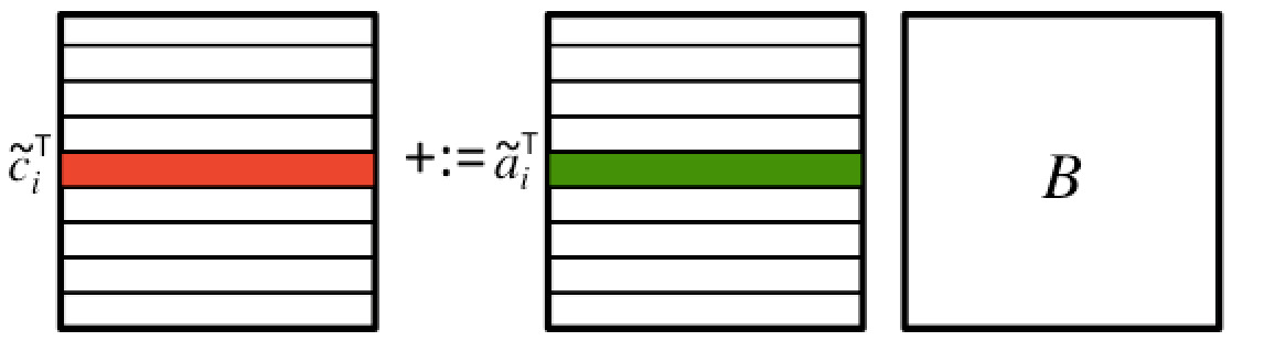
This illustrates how the IJP and IPJ algorithms can be viewed as a loop around the updating of a row of \(C \) with the product of the corresponding row of \(A \) times matrix \(B \text{:}\)

\begin{equation*} \begin{array}{l} \begin{array}{l} {\bf for~} i := 0, \ldots , m-1 \\[0.15in] ~~~ \left. \begin{array}{l} {\bf for~} j := 0, \ldots , n-1 \\[0.15in] ~~~ ~~~ \left. \begin{array}{l} {\bf for~} p := 0, \ldots , k-1 \\ ~~~ ~~~ \gamma_{i,j} := \alpha_{i,p} \beta_{p,j} + \gamma_{i,j} \\ {\bf end} \end{array} \right\} ~~~ \widetilde \gamma_{i,j} := \widetilde a_i^T b_j + \widetilde \gamma_{i,j} \\[0.2in] ~~~ {\bf end} \end{array} \right\} ~~~ \widetilde c_i^T := \widetilde a_i^T B + \widetilde c_i^T \\[0.2in] {\bf end} \end{array} \end{array} \end{equation*}

and

\begin{equation*} \begin{array}{l} \begin{array}{l} {\bf for~} i := 0, \ldots , m-1 \\[0.15in] ~~~ \left. \begin{array}{l} {\bf for~} p := 0, \ldots , k-1 \\[0.15in] ~~~ ~~~ \left. \begin{array}{l} {\bf for~} j := 0, \ldots , n-1 \\ ~~~ ~~~ \gamma_{i,j} := \alpha_{i,p} \beta_{p,j} + \gamma_{i,j} \\ {\bf end} \end{array} \right\} ~~~ \widetilde c_i^T := \alpha_{i,p} \widetilde b_p^T + \widetilde c_i^T \\[0.2in] ~~~ {\bf end} \end{array} \right\} ~~~ \widetilde c_i^T := \widetilde a_i^T B + \widetilde c_i^T \\[0.2in] {\bf end} \end{array} \end{array} \end{equation*}

The problem with implementing the above algorithms is that Gemv_I_Dots and Gemv_J_Axpy implement \(y := A x + y \) rather than \(y^T := x^T A + y^T \text{.}\) Obviously, you could create new routines for this new operation. We will instead look at how to use the BLAS and BLIS interfaces.

Recall that the BLAS include the routine dgemv that computes

\begin{equation*} y := \alpha A x + \beta y \quad \mbox{or} \quad y := \alpha A^T x + \beta y. \end{equation*}

What we want is a routine that computes

\begin{equation*} y^T := x^T A + y^T. \end{equation*}
\(A = B \)\(A^T = B^T \text{,}\)\(( A + B)^T = A^T + B^T \text{,}\)\((A B)^T = B^T A^T \text{.}\)
\begin{equation*} y^T = x^T A + y^T, \end{equation*}
\begin{equation*} (y^T)^T = ( x^T A + y^T)^T \end{equation*}
\begin{equation*} y = ( x^T A )^T + (y^T)^T \end{equation*}

and finally

\begin{equation*} y = A^T x + y. \end{equation*}

So, updating

\begin{equation*} y^T := x^T A + y^T \end{equation*}
\begin{equation*} y := A^T x + y. \end{equation*}

It this all seems unfamiliar, you may want to look at Linear Algebra: Foundations to Frontiers

Now, if

  • \(m \times n \) matrix \(A \) is stored in array A with its leading dimension stored in variable ldA,

  • \(m \) is stored in variable m and \(n \) is stored in variable n,

  • vector \(x \) is stored in array x with its stride stored in variable incx,

  • vector \(y \) is stored in array y with its stride stored in variable incy, and

  • \(\alpha \) and \(\beta \) are stored in variables alpha and beta, respectively,

then \(y := \alpha A^T x + \beta y \) translates, from C, into the call

dgemv_( "Transpose", &m, &n, &alpha, A, &ldA, x, &incx, &beta, y, &incy );

The BLIS native call that is similar to the BLAS dgemv routine in this setting translates to

bli_dgemv( BLIS_TRANSPOSE, BLIS_NO_CONJUGATE, m, n,
&alpha, A, ldA, 1, x, incx, &beta, y, incy );

Because of the two parameters after A that capture the stride between elements in a column (the row stride) and elements in rows (the column stride), one can alternatively swap these parameters:

bli_dgemv( BLIS_NO_TRANSPOSE, BLIS_NO_CONJUGATE, m, n,
&alpha, A, ldA, 1, x, incx, &beta, y, incy );

Unit 1.4.6 Discussion

The point of this section is that one can think of matrix-matrix multiplication as one loop around

  • multiple matrix-vector multiplications:

    \begin{equation*} \left( \begin{array}{c | c | c } c_0 \amp \cdots \amp c_{n-1} \end{array} \right) = \left( \begin{array}{c | c | c } A b_0 + c_0 \amp \cdots \amp A b_{n-1} + c_{n-1} \end{array} \right) \end{equation*}
  • multiple rank-1 updates:

    \begin{equation*} C = a_0 \widetilde b_0^T + a_1 \widetilde b_1^T + \cdots + a_{k-1} \widetilde b_{k-1}^T + C \end{equation*}
  • multiple row times matrix multiplications:

    \begin{equation*} \left( \begin{array}{c} \widetilde c_0^T \\ \hline \widetilde c_1^T \\ \hline \vdots \\ \hline \widetilde c_{m-1}^T \end{array} \right) = \left( \begin{array}{c} \widetilde a_0^T B + \widetilde c_0^T \\ \hline \widetilde a_1^T B + \widetilde c_1^T \\ \hline \vdots \\ \hline \widetilde a_{m-1}^T B + \widetilde c_{m-1}^T \end{array} \right) \end{equation*}

So, for the outer loop there are three choices: \(j \text{,}\) \(p \text{,}\) or \(i \text{.}\) This may give the appearance that there are only three algorithms. However, the matrix-vector multiply and rank-1 update hide a double loop and the order of these two loops can be chosen, to bring us back to six choices for algorithms. Importantly, matrix-vector multiplication can be organized so that matrices are addressed by columns in the inner-most loop (the JI order for computing gemv) as can the rank-1 update (the JI order for computing ger). For the implementation that picks the I loop as the outer loop, gemv is utilized but with the transposed matrix. As a result, there is no way of casting the inner two loops in terms of operations with columns.
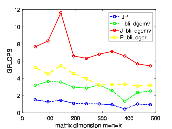
Figure 1.4.4 Left: Performance of simple implementations of the different loop orderings. Right: Performance for different choices of the outer loop, calling the BLIS typed interface. All experiments were performed on Robert's laptop. Notice that the scale along the y-axis is not consistent between the two graphs.
Homework 1.4.19

In directory Assignments/Week1/C/data use the Live Script in /Assignments/Week1/C/data/Plot_All_Outer.mlx to compare and contrast the performance of many of the algorithms that use the I, J, and P loop as the outer-most loop. If you want to rerun all the experiments, you can do so by executing

make Plot_All_Outer

in directory Assignments/Week1/C. What do you notice?

From the performance experiments reported in Figure 1.4.4, we have observed that accessing matrices by columns, so that the most frequently loaded data is contiguous in memory, yields better performance. Still, the observed performance is much worse than can be achieved.

We have now partitioning the matrices ,what we call "slicing and dicing", enhances our insight into how different algorithms access data. This will be explored and exploited further in future weeks.