Section 2.4 Optimizing the Microkernel
¶Unit 2.4.1 Reuse of Data in Registers
¶In Section 2.3 we introduced the fact that modern architectures have vector registers and then showed how to (somewhat) optimize the update of a \(4 \times 4 \) submatrix of \(C \text{.}\)
Some observations:
The block is \(4 \times 4 \text{.}\) In general, the block is \(m_R \times n_R \text{,}\) where in this case \(m_R = n_R = 4 \text{.}\) If we assume we will use \(R_C \) registers for elements of the submatrix of \(C \text{,}\) what should \(m_R \) and \(n_R \) be, given the constraint that \(m_R \times n_R \leq R_C \text{?}\)
Given that some registers need to be used for elements of \(A \) and \(B \text{,}\) how many registers should be used for elements of each of the matrices? In our implementation in the last section, we needed one vector register for four elements of \(A \) and one vector register in which one element of \(B \) is broadcast (duplicated). Thus, \(16 + 4 + 1 \) elements of matrices were being stored in \(6 \) out of \(16\) available vector registers.
What we notice is that, ignoring the cost of loading and storing elements of \(C \text{,}\) loading four doubles from matrix \(A \) and broadcasting four doubles from matrix \(B \) is amortized over 32 flops. The ratio is \(32\) flops for \(8 \) loads, or \(4~~ {\rm flops}/{\rm load} \text{.}\) Here for now we ignore the fact that loading the four elements of \(A \) is less costly than broadcasting the four elements of \(B \text{.}\)
Unit 2.4.2 More options
¶Modify Assignments/Week2/C/Gemm_JI_4x4Kernel.c to implement the case where \(m_R = 8 \) and \(n_R =
4 \text{,}\) storing the result in Gemm_JI_8x4Kernel.c. Don't forget to update MR and NR! You can test the result by typing
make JI_8x4Kernelin that directory and view the resulting performance by appropriately modifying
Assignments/Week2/C/data/Plot_MRxNR_Kernels.mlx.Homework 2.4.2
How many vector registers are needed for the implementation in Homework 2.4.1?
Ignoring the cost of loading the registers with the \(8 \times 4 \) submatrix of \(C \text{,}\) analyze the ratio of flops to loads for the implementation in Homework 2.4.1.
Solution
Number of registers:
\begin{equation*}
8 + 3 = 11
\end{equation*}
Ratio:
\begin{equation*}
64 flops/12 loads \approx 5.33 flops/load.
\end{equation*}
Homework 2.4.3
We have considered \(m_R \times n_R = 4 \times 4 \) and \(m_R \times n_R = 8 \times 4 \text{,}\) where elements of \(A \) are loaded without duplication into vector registers (and hence \(m_R \) must be a multiple of \(4 \)), and elements of \(B \) are loaded/broadcast. Extending this approach to loading \(A \) and \(B \text{,}\) complete the entries in the following table:
\begin{equation*}
\begin{array}{| c | c | c |} \hline
\amp {\rm \#~of~vector~regs}
\amp {\rm flops/load} \\ \hline
4 \times 1 \amp ~~~~ \amp ~~~ / ~~~ = ~~~~~~ \\ \hline
4 \times 2 \amp ~~~~ \amp ~~~ / ~~~ = ~~~~~~ \\ \hline
4 \times 4 \amp 6 \amp 32 / 8 = 4 \\ \hline
4 \times 8 \amp ~~~~ \amp ~~~ / ~~~ = ~~~~~~~ \\ \hline
4 \times 12 \amp ~~~~ \amp ~~~ / ~~~ = ~~~~~~ \\ \hline
4 \times 14 \amp ~~~~ \amp ~~~ / ~~~ = ~~~~~~ \\ \hline
8 \times 1 \amp ~~~~ \amp ~~~ / ~~~ = ~~~~~~ \\ \hline
8 \times 2 \amp ~~~~ \amp ~~~ / ~~~ = ~~~~~~ \\ \hline
8 \times 4 \amp ~~~~ \amp ~~~ / ~~~ = ~~~~~~ \\ \hline
8 \times 6 \amp ~~~~ \amp ~~~ / ~~~ = ~~~~~~ \\ \hline
8 \times 8 \amp ~~~~ \amp ~~~ / ~~~ = ~~~~~~ \\ \hline
12 \times 1 \amp ~~~~ \amp ~~~ / ~~~ = ~~~~~~ \\ \hline
12 \times 2 \amp ~~~~ \amp ~~~ / ~~~ = ~~~~~~ \\ \hline
12 \times 4 \amp ~~~~ \amp ~~~ / ~~~ = ~~~~~~ \\ \hline
12 \times 6 \amp ~~~~ \amp ~~~ / ~~~ = ~~~~~~ \\ \hline
\end{array}
\end{equation*}
Solution
Fix!
\begin{equation*}
\begin{array}{| c | c | r |} \hline
\amp {\rm \#~of~vector~regs}
\amp {\rm flops/load} \\ \hline
4 \times 1 \amp 3 \amp 8 / ~5 = 1.60 \\ \hline
4 \times 2 \amp 4 \amp 16 / ~6 = 2.66 \\ \hline
4 \times 4 \amp 6 \amp 32 /~ 8 = 4.00 \\ \hline
4 \times 8 \amp 10 \amp 64/12 = 5.44 \\ \hline
4 \times 12 \amp 14 \amp 96 / 16 = 6.00 \\ \hline
4 \times 14 \amp 16 \amp 112 / 18 = 6.22 \\ \hline
8 \times 1 \amp 5 \amp 16 / ~9 = 1.78 \\ \hline
8 \times 2 \amp 7 \amp 32 / 10 = 3.20 \\ \hline
8 \times 4 \amp 11 \amp 64 / 12 = 5.33 \\ \hline
8 \times 6 \amp 15 \amp 96 /14 = 6.86 \\ \hline
8 \times 8 \amp 67 \amp 128 /16 = 8.00 \\ \hline
12 \times 1 \amp 7 \amp 24 / 13 = 1.85 \\ \hline
12 \times 2 \amp 10 \amp 48 /14 = 3.43 \\ \hline
12 \times 4 \amp 16 \amp 96 /16 = 6.00 \\ \hline
12 \times 6 \amp 22 \amp 144 /18 = 8.00 \\ \hline
\end{array}
\end{equation*}
Homework 2.4.4
At this point, you have already implemented the following kernels: Gemm_JI_4x4Kernel.c and Gemm_JI_8x4Kernel.c. Implement as many of the more promising of the kernels you analyzed in the last homework as you like. They can be executed by typing
make test_JI_?x?Kernelwhere the ?'s are replaced with the obvious choices of \(m_R \) and \(n_R \text{.}\) Don't forget to update MR and NR! The resulting performance can again be viewed with Live Script in
Assignments/Week2/C/data/Plot_MRxNR_Kernels.mlx }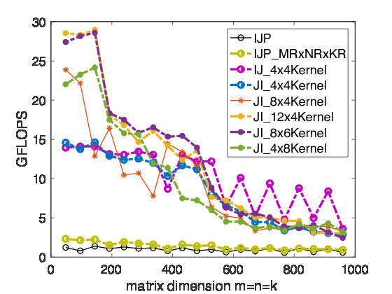
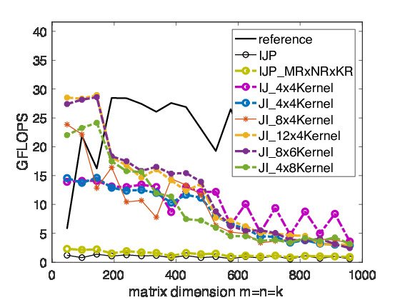
In Figure 2.4.5, we show the performance of matrix-matrix multiplication cast in terms of various microkernel calls on Robert's laptop.
Unit 2.4.3 Amortizing data movement
¶As we have already discussed, one of the fundamental principles behind high performance is that when data is moved from one layer of memory to another, one needs to amortize the cost of that data movement over many computations. In our discussion so far, we have only discussed two layers of memory: (vector) registers and a cache.
Let us focus on the current approach:
Four vector registers are loaded with a \(m_R \times n_R\) submatrix of \(C \text{.}\) The cost of loading and unloading this data is negligible if \(k \) size is large.
\(m_R / 4 \) vector register is loaded with the current column of \(A \text{,}\) with \(m_R \) elements. In our picture, we call this register alpha_0123_p. The cost of this load is amortized over \(2 m_R \times n_R \) floating point operations.
One vector register is loaded with broadcast elements of the current row of \(B \text{.}\) The loading of the \(n_R \) of the elements is also amortized over \(2 m_R \times n_R\) floating point operations.
To summarize, ignoring the cost of loading the submatrix of \(C \text{,}\) this would then require
\begin{equation*}
m_R + n_R
\end{equation*}
floating point number loads from slow memory, \(m_R\) elements of \(A \) and \(n_R \) elements of \(B \text{,}\) which are amortized over \(2 \times m_R \times n_R \) flops, for each rank-1 update.
If loading a double as part of vector load costs the same as the loading and broadcasting of a double, then the problem of finding the optimal choices of \(m_R \) and \(n_R \) can be stated as finding the \(m_R \) and \(n_R \) that optimize
\begin{equation*}
\frac{2 m_R n_R}{m_R + n_R}
\end{equation*}
under the constraint that
\begin{equation*}
m_R n_R + m_R + 1 = r_C,
\end{equation*}
where \(r_c \) equals the number of doubles that can be stored in vector registers.
Finding the optimal solution is somewhat nasty, even if \(m_R\) and \(n_R \) are allowed to be real valued rather than integers. If we recognize that \(m_R + 1 \) is small relative to \(m_R n_R \text{,}\) and therefore ignore that those need to be kept in registers, we instead end up with having to find the \(m_R \) and \(n_R \) that optimize
\begin{equation*}
\frac{2 m_R n_R}{m_R + n_R}
\end{equation*}
under the constraint that
\begin{equation*}
m_R n_R = r_C.
\end{equation*}
This is essentially a standard problem in calculus, used to find the sides of the rectangle with length \(x \) and width \(y\) that maximizes the area of the rectangle, \(xy \text{,}\) under the constraint that the length of the perimeter is constant. The answer for that problem is that the rectangle should be a square. Thus, we want the submatrix of \(C \) that is kept in registers to be "squarish."
In practice, we have seen that the shape of the block of \(C\) kept in registers is noticeably not square. The reason for this is that, all other issues being equal, loading a double as part of a vector load requires fewer cycles than loading a double as part of a load/broadcast.
Unit 2.4.4 Discussion
¶Notice that we have analyzed that we must amortize the loading of elements of \(A \) and \(B\) over, at best, a few flops per such element. The "latency" from main memory (the time it takes for a double precision number to be fetched from main memory) is equal to the time it takes to perform on the order of 100 flops. Thus, "feeding the beast" from main memory spells disaster. Fortunately, modern architectures are equipped with multiple layers of cache memories that have a lower latency.
In Figure 2.4.5, we saw that for small matrices that fit in the L-2 cache, performance is very good, especially for the right choices of \(m_R \times n_R \text{.}\) The performance drops when problem sizes spill out of the L2 cache and drops again when they spill out of the L3 cache.