Section 4.4 Parallelizing More
¶Unit 4.4.1 Speedup, efficiency, etc.
¶Amdahl's law is a simple observation regarding how much speedup can be expected when one parallelizes a code. First some definitions.
-
Sequential time.
The sequential time for an operation is given by
\begin{equation*} T( n ), \end{equation*}where \(n \) is a parameter that captures the size of the problem being solved. For example, if we only time problems with square matrices, then \(n \) would be the size of the matrices. \(T(n) \) is equal the time required to compute the operation on a single core.
-
Parallel time.
The parallel time for an operation and a given implementation using \(t \) threads is given by
\begin{equation*} T_t( n ). \end{equation*} -
Speedup.
The speedup for an operation and a given implementation using \(t \) threads is given by
\begin{equation*} T( n ) / T_t( n ). \end{equation*}It measures how much speedup is attained by using \(t \) threads. Generally speaking, it is assumed that
\begin{equation*} S_t( n ) = T( n ) / T_t( n ) \leq t . \end{equation*}This is not always the case: sometimes \(t \) threads collective have resources (e.g., more cache memory) that allows speedup to exceed \(t \text{.}\) Think of the case where you make a bed with one person versus two people: You can often finish the job more than twice as fast because two people do not need to walk back and forth from one side of the bed to the other.
-
Efficiency.
The efficiency for an operation and a given implementation using \(t \) threads is given by
\begin{equation*} S_t(n) / t . \end{equation*}It measures how efficiently the \(t \) threads are being used.
-
GFLOPS.
We like to report GFLOPS (billions of floating point operations per second). Notice that this gives us an easy way of judging efficiency: If we know what the theoretical peak of a core is, in terms of GFLOPS, then we can easily judge how efficiently we are using the processor relative to the theoretical peak. How do we compute the theoretical peak? We can look up the number of cycles a core can perform per second and the number of floating point operations it can before per cycle. This can then be converted to a peak rate of computation for a single core (in billions of floating point operations per second). If there are multiple cores, we just multiply this peak by the number of cores.
Of course, this is all complicated by the fact that as more cores are utilized, each core often executes at a lower clock speed so as to keep the processor from overheating.
Unit 4.4.2 Ahmdahl's law
¶Ahmdahl's law is a simple observation about the limits on parallel speed and efficiency. Consider an operation that requires sequential time
\begin{equation*}
T
\end{equation*}
for computation. What if fraction \(f \) of this time is {\bf not} parallelized, and the other fraction \((1-f)\) is parallelized with \(t \) threads. Then the total execution time is
\begin{equation*}
T_t \geq (1-f) T / t + f T.
\end{equation*}
This, in turn, means that the speedup is bounded by
\begin{equation*}
S \leq \frac{T}{(1-f) T / t + f T}.
\end{equation*}
Now, even if the parallelization with \(t \) threads is such that the fraction that is being parallelized takes no time at all (\((1-f) T/ t = 0 \)), then we still find that
\begin{equation*}
S \leq \frac{T}{(1-f) T / t + f T}
\leq \frac{T}{(f T} = \frac{1}{f}.
\end{equation*}
What we notice is that the maximal speedup is bounded by the inverse of the fraction of the execution time that is not parallelized. So, if 20% of the code is not optimized, then no matter how many threads you use, you can at best compute the result five times faster. This means that one must think about parallelizing all significant parts of a code.
Ahmdahl's law says that if does not parallelize the part of a sequential code in which fraction \(f \) time is spent, then the speedup attained regardless of how many threads are used is bounded by \(1/f \text{.}\)
The point is: So far, we have focused on parallelizing the computational part of matrix-matrix multiplication. We should also parallelize the packing, since that is a nontrivial part of the total execution time.
Unit 4.4.3 Parallelizing the packing
¶Some observations:
If you choose to parallelize Loop 3 around the microkernel, then the packing into \(\widetilde A \) is already parallelized, since each thread packs its own such block. So, you will want to parallelize the packing of \(\widetilde B \text{.}\) If you choose to parallelize Loop 2 around the microkernel, you will also want to parallelize the packing of \(\widetilde A \text{.}\)
Be careful: we purposely wrote the routines that pack \(\widetilde A \) and \(\widetilde B \) so that a naive parallelization will give the wrong answer. Analyze carefully what happens when multiple threads execute the loop...
In directory Week4/C,
Copy Gemm_Parallel_Loop2_12x4.c into Gemm_Parallel_Loop2_Parallel_Pack_12x4.c.
Parallelize the packing of \(\widetilde B \) and/or \(\widetilde A \text{.}\)
Set the number of threads to some number between \(1 \) and the number of CPUs in the target processor.
Execute
make Parallel_Loop2_Parallel_Pack_12x4
.View the resulting performance with ShowPerformance.mlx, uncommenting the appropriate lines.
Be sure to check if you got the right answer! This actually is trickier than you might at first think!