LAFF-On Programming for High Performance

Unit 1.3.1 The Basic Linear Algebra Subprograms (BLAS)

Linear algebra operations are fundamental to computational science. In the 1970s, when vector supercomputers reigned supreme, it was recognized that if applications and software libraries are written in terms of a standardized interface to routines that implement operations with vectors, and vendors of computers provide high-performance instantiations for that interface, then applications would attain portable high performance across different computer platforms. This observation yielded the original Basic Linear Algebra Subprograms (BLAS) interface [3] for Fortran 77, which are now referred to as the level-1 BLAS. The interface was expanded in the 1980s to encompass matrix-vector operations (level-2 BLAS)~\cite{BLAS2} and matrix-matrix operations (level-3 BLAS) [1].

An overview of the BLAS and how they are used to achieve portable high performance is given in the Encyclopedia of Parallel Computing [5]. This article is somewhat out of date. In a later enrichment we will point you to the BLAS-like Library Instantiation Software (BLIS) [6], which is now a widely used open source framework for rapidly instantiating the BLAS and similar functionality.

Expressing code in terms of the BLAS has another benefit: the call to the routine hides the loop that otherwise implements the vector-vector operation and clearly reveals the operation being performed, thus improving readability of the code.

Unit 1.3.2 Notation

In our discussions, we use capital letters for matrices (\(A, B, C, \ldots \)), lower case letters for vectors (\(a, b, c, \ldots \)), and lower case Greek letters for scalars (\(\alpha, \beta, \gamma, \ldots \)). Exceptions are integer scalars, for which we will use \(i, j, k, m, n,\) and \(p \text{.}\)

Vectors in our universe are column vectors or, equivalently, \(n \times 1 \) matrices if the vector has \(n \) components (size \(n \)). A row vector we view as a column vector that has been transposed. So, \(x \) is a column vector and \(x^T \) is a row vector.

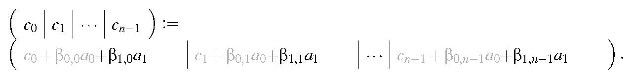
In the subsequent discussion, we will want to expose the rows or columns of a matrix. If \(X \) is an \(m \times n\) matrix, then we expose its columns as

so that \(x_j \) equals the column with index \(j \text{.}\) We expose its rows as

so that \(\widetilde x_i^T \) equals the row with index \(i \text{.}\) Here the \(~^T\) indicates it is a row (a column vector that has been transposed). The tilde is added for clarity since \(x_i^T \) would in this setting equal the column indexed with \(i \) that has been transposed, rather than the row indexed with \(i \text{.}\) When there isn't a cause for confusion, we will sometimes leave the \(\widetilde ~\) off. We use the lower case letter that corresponds to the upper case letter used to denote the matrix, as an added visual clue that \(x_j \) is a column of \(X \) and \(\widetilde x_i^T \) is a row of \(X \text{.}\)

We have already seen that the scalars that constitute the elements of a matrix or vector are denoted with the lower Greek letter that corresponds to the letter used for the matrix of vector:

If you look carefully, you will notice the difference between \(x \) and \(\chi \text{.}\) The latter is the lower case Greek letter "chi."

Unit 1.3.3 The dot product (inner product)

Given two vectors \(x \) and \(y \) of size \(n \)

their dot product is given by

The notation \(x^T y \) comes from the fact that the dot product also equals the result of multiplying \(1 \times n\) matrix \(x^T \) times \(n \times 1 \) matrix \(y \text{.}\)

A routine. coded in C, that computes \(x^T y + \gamma \) where \(x \) and \(y \) are stored at location x with stride incx and location y with stride incy, respectively, and \(\gamma \) is stored at location gamma is given by

#define chi( i ) x[ (i)*incx ]   // map chi( i ) to array x 
#define psi( i ) y[ (i)*incy ]   // map psi( i ) to array y

void Dots( int n, double *x, int incx, double *y, int incy, double *gamma )
{
  for ( int i=0; i<n; i++ )
    *gamma += chi( i ) * psi( i );
}

The BLAS include a function for computing the dot operation. Its calling sequence in Fortran, for double precision data, is

DDOT( N, X, INCX, Y, INCY )

• (input) N is an integer that equals the size of the vectors.

• (input) X is the address where \(x \) is stored.

• (input) INCX is the stride in memory between entries of \(x \text{.}\)

• (input) Y is the address where \(y \) is stored.

• (input) INCYnnnn is the stride in memory between entries of \(y \text{.}\)

The function returns the result as a scalar of type double precision. If the datatype were single precision, complex double precision, or complex single precision, then the first D is replaced by S, Z, or C, respectively.

To call the same routine in a code written in C, it is important to keep in mind that Fortran passes data by address. The call

Dots( n, x, incx, y, incy, &gamma );

gamma += ddot_( &n, x, &incx, y, &incy );

Dots( n, x, 1, y, incy, &gamma );

int i_one=1;
gamma += ddot_( &n, x, &i_one, y, &incy );

In this course, we use the BLIS implementation of the BLAS as our library. This library also has its own (native) BLAS-like interface that we refer to as the BLIS Typed API. (BLIS is actually a framework for the rapid instantiation of BLAS-like functionality. It comes with four different interfaces to that functionality: The classic Fortran BLAS interface, the CBLAS interface for the C language (which is an interface that is rarely used), the BLIS Typed API with is reminiscent of the BLAS interface, but with added functionality and flexibility, and the BLIS object API, which which a Users' Guide can be found at https://github.com/flame/blis/blob/master/docs/BLISObjectAPI.md.) A Users' Guide for this interface can be found at https://github.com/flame/blis/blob/master/docs/BLISTypedAPI.md. There, we find the routine bli_ddotxv that computes \(\gamma := \alpha x^T y + \beta \gamma \text{,}\) optionally conjugating the elements of the vectors. The call

Dots( n, x, incx, y, incy, &gamma );

double one=1.0;    
bli_ddotxv( BLIS_NO_CONJUGATE, BLIS_NO_CONJUGATE,
            n, &one, x, incx, y, incy, &one, &gamma );

Unit 1.3.4 The IJP and JIP orderings

Let us return once again to the IJP ordering of the loops that compute matrix-matrix multiplication:

This pseudo-code translates into the routine coded in C given in Figure 1.1.1.

We then notice that

If this makes your head spin, you will want to quickly go through Weeks 3-5 of our MOOC titled "Linear Algebra: Foundations to Fontiers,.'' which is an introductory undergraduate course. It captures that the outer two loops visit all of the elements in \(C \text{,}\) and the inner loop implements the dot product of the appropriate row of \(A \) with the appropriate column of \(B \text{:}\) \(\gamma_{i,j} := \widetilde a_i^T b_j + \gamma_{i,j} \text{,}\) as illustrated by

which is, again, the IJP ordering of the loops.

Obviously, one can equally well switch the order of the outer two loops, which just means that the elements of \(C \) are computed a column at a time rather than a row at a time:

make JI_Dots
make JI_ddot
make JI_bli_ddotxv

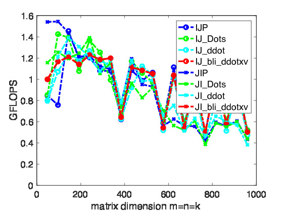
In Figure~\ref{fig:IJP_JIP} we report the performance of the various implementations from the last homeworks. What we notice is that, at least when using Apple's clang compiler, not much difference results from hiding the inner-most loop in a subroutine.

Unit 1.3.5 The axpy operations

Given a scalar, \(\alpha \text{,}\) and two vectors, \(x \) and \(y \text{,}\) of size \(n \) with elements

which in terms of the elements of the vectors equals

The name axpy comes from the fact that in Fortran 77 only six characters and numbers could be used to designate the names of variables and functions. The operation \(\alpha x + y \) can be read out loud as "scalar apha times x plus y" which yields the acronym axpy.

An outline for a routine that implements the axpy operation is given by

#define chi( i ) x[ (i)*incx ]   // map chi( i ) to array x 
#define psi( i ) y[ (i)*incy ]   // map psi( i ) to array y

void Axpy( int n, double alpha, double *x, int incx, double *y, int incy )
{
  for ( int i=0; i<n; i++ )
    psi(i)  += 
}

in file Assignments/Week1/C/Axpy.c.

The BLAS include a function for computing the axpy operation. Its calling sequence in Fortran, for double precision data, is

DAXPY( N, ALPHA, X, INCX, Y, INCY )

where

• (input) N is the address of the integer that equals the size of the vectors.

• (input) ALPHA is the address where \(\alpha \) is stored.

• (input) X is the address where \(x \) is stored.

• (input) INCX is the address where the stride between entries of \(x \) is stored.

• (input/output) Y is the address where \(y \) is stored.

• (input) INCY is the address where the stride between entries of \(y \) is stored.

It may appear strange that the addresses of N, ALPHA, INCX, and INCY are passed in. This is because Fortran passes parameters by address rather than value.) If the datatype were single precision, complex double precision, or complex single precision, then the first D is replaced by S, Z, or C, respectively.

In C, the call

Axpy( n, alpha, x, incx, y, incy );

translates to

daxpy_( &n, &alpha, x, &incx, y, &incy );

which links to the Fortran interface. Notice that the scalar parameters n, alpha, incx, and incy are passed "by address" because Fortran passes parameters to subroutines by address. We will see examples of its use later in this section.

The BLIS native routine for axpy is bli_dapyv. The call

Axpy( n, alpha, x, incx, y, incy );

bli_daxpyv( BLIS_NO_CONJUGATE, n, alpha, x, incx, y, incy );

The BLIS_NO_CONJUGATE is to indicate that vector \(x \) is not to be conjugated. That parameter is there for consistency with the complex versions of this routine (bli_zaxpyv and bli_caxpyv).

In an implementation of the algorithm for computing \(C := A B + C \) given by

and illustrated by

one can now replace the loop indexed by \(j \) with a call to Axpy.

#define alpha( i,j ) A[ (j)*ldA + i ]   // map alpha( i,j ) to array A 
#define beta( i,j )  B[ (j)*ldB + i ]   // map beta( i,j )  to array B
#define gamma( i,j ) C[ (j)*ldC + i ]   // map gamma( i,j ) to array C

void Axpy( int, double, double *, int, double *, int );

void MyGemm( int m, int n, int k, double *A, int ldA,
	     double *B, int ldB, double *C, int ldC )
{
  for ( int i=0; i<m; i++ )
    for ( int p=0; p<k; p++ )
      Axpy( n, alpha( i,p ), &beta( p,0 ), ldB, &gamma( i,0 ), ldC );
}

Unit 1.3.6 The IPJ and PIJ orderings

What we notice is that there are \(3! \) ways of order the loops: Three choices for the outer loop, two for the second loop, and one choice for the final loop. Let's consider the IPJ ordering:

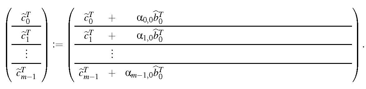
One way to think of the above algorithm is to view matrix \(C \) as its rows, matrix \(A \) as its individual elements, and matrix \(B\) as its rows:

We then notice that

This captures that the outer two loops visit all of the elements in \(A \text{,}\) and the inner loop implements the updating of the \(i \)th row of \(C \) by adding \(\alpha_{i,p} \) times the \(p \)th row of \(B \) to it, as captured by

make IP_Axpy

make IP_daxpy

make IP_bli_daxpyv

One can switch the order of the outer two loops to get

The outer loop in this second algorithm fixes the row of \(B\) that is used to to update all rows of \(C \text{,}\) using the appropriate element from \(A \) to scale. In the first iteration of the outer loop (\(p = 0 \)), the following computations occur:

make PI_Axpy
make PI_daxpy 
make PI_bli_daxpyv

Unit 1.3.7 The JPI and PJI orderings

Let us consider the JPI ordering:

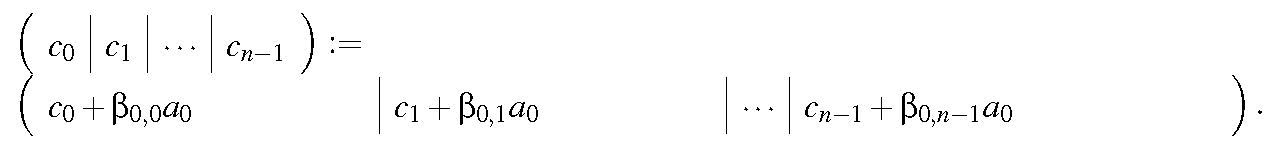
Another way to think of the above algorithm is to view matrix \(C \) as its columns, matrix \(A \) as its columns, and matrix \(B \) as its individual elements. Then

so that

The algorithm captures this as

make JP_Axpy

make JP_daxpy

make JP_bli_daxpyv

One can switch the order of the outer two loops to get

The outer loop in this algorithm fixes the column of \(A \) that is used to to update all columns of \(C \text{,}\) using the appropriate element from \(B \) to scale. In the first iteration of the outer loop, the following computations occur:

make PJ_Axpy 
make PJ_daxpy 
make PJ_bli_daxpyv

The purpose of this section was mostly to help you think in terms of operations with vectors (the rows and columns of the matrices) when reasoning about, and implementing, the inner-most loop of the different algorithms for computing a matrix-matrix multiplication. On Robert's laptop, the performance is not much affected. For this reason, in the below exercise, we revisit the performance graphs for the different loop orderings from Section~\ref{sec:AllOrderings}.

Unit 1.3.8 Discussion

Homework 1.3.15

In Figure 1.3.3, the results of Homework 1.2.5 on Robert's laptop are again reported. What do the two loop orderings that result in the best performances have in common? You may want to use the following worksheet to answer this question:

Solution

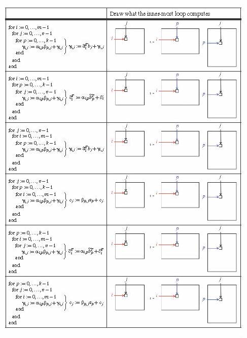
They both have the loop indexed with \(i \) as the inner-most loop and that loop computes with columns of \(C \) and \(A \text{.}\)